British Library Cataloguing in Publication Data
A catalogue record for this book is available from the British Library. ISBN-13: 978-1-59693-238-8
Cover design by Yekaterina Ratner 2008 ARTECH HOUSE, INC. 685 Canton Street
Norwood, MA 02062
All rights reserved. Printed and bound in the United States of America. No part of this book may be reproduced or utilized in any form or by any means, electronic or mechanical, including photocopying, recording, or by any information storage and retrieval system, without permission in writing from the publisher.
All terms mentioned in this book that are known to be trademarks or service marks have been appropriately capitalized. Artech House cannot attest to the accuracy of this information. Use of a term in this book should not be regarded as affecting the validity of any trademark or service mark.
Preface xiii
1 Introduction 1
1.1 What Is IBE? 1
1.2 Why Should I Care About IBE? 8
References 13
2 Basic Mathematical Concepts and Properties 15
2.1 Concepts from Number Theory 15
2.1.1 Computing the GCD 16
2.1.2 Computing Jacobi Symbols 24
2.2 Concepts from Abstract Algebra 25
References 39
3 Properties of Elliptic Curves 41
3.1 Elliptic Curves 41
3.2 Adding Points on Elliptic Curves 47
3.2.1 Algorithm for Elliptic Curve Point Addition 52
3.2.2 Projective Coordinates 53
3.2.3 Adding Points in Jacobian Projective Coordinates 54
3.2.4 Doubling a Point in Jacobian Projective
Coordinates 55
3.3 Algebraic Structure of Elliptic Curves 55
3.3.1 Higher Degree Twists 61
3.3.2 Complex Multiplication 65
References 66
4 Divisors and the Tate Pairing 67
4.1 Divisors 67
4.1.1 An Intuitive Introduction to Divisors 68
4.2 The Tate Pairing 76
4.2.1 Properties of the Tate Pairing 81
4.3 Miller’s Algorithm 84
References 87
5 Cryptography and Computational Complexity 89
5.1 Cryptography 91
5.1.1 Definitions 91
5.1.2 Protection Provided by Encryption 93
5.1.3 The Fujisaki-Okamoto Transform 95
5.2 Running Times of Useful Algorithms 95
5.2.1 Finding Collisions for a Hash Function 96
5.2.2 Pollard’s Rho Algorithm 98
5.2.3 The General Number Field Sieve 99
5.2.4 The Index Calculus Algorithm 102
5.2.5 Relative Strength of Algorithms 102
5.3 Useful Computational Problems 104
5.3.1 The Computational Diffie-Hellman Problem 105 5.3.2 The Decision Diffie-Hellman Problem 106 5.3.3 The Bilinear Diffie-Hellman Problem 107 5.3.4 The Decision Bilinear Diffie-Hellman Problem 107 5.3.5 q-Bilinear Diffie-Hellman Inversion 108 5.3.6 q-Decision Bilinear Diffie-Hellman Inversion 109
5.3.8 Integer Factorization 109
5.3.9 Quadratic Residuosity 109
5.4 Selecting Parameter Sizes 110
5.4.1 Security Based on Integer Factorization and
Quadratic Residuosity 110
5.4.2 Security Based on Discrete Logarithms 110
5.5 Important Special Cases 111
5.5.1 Anomalous Curves 112
5.5.2 Supersingular Elliptic Curves 112
5.5.3 Singular Elliptic Curves 113
5.5.4 Weak Primes 113
5.6 Proving Security of Public-Key Algorithms 114
5.7 Quantum Computing 116
5.7.1 Grover’s Algorithm 116
5.7.2 Shor’s Algorithm 117
References 118
6 Related Cryptographic Algorithms 121
6.1 Goldwasser-Michali Encryption 121
6.2 The Diffie-Hellman Key Exchange 124
6.3 Elliptic Curve Diffie-Hellman 125
6.4 Joux’s Three-Way Key Exchange 126
6.5 ElGamal Encryption 128
References 129
7 The Cocks IBE Scheme 131
7.1 Setup of Parameters 131
7.2 Extraction of the Private Key 133
7.3 Encrypting with Cocks IBE 133
7.4 Decrypting with Cocks IBE 135
7.6 Security of the Cocks IBE Scheme 139 7.6.1 Relationship to the Quadratic Residuosity
Problem 139
7.6.2 Chosen Ciphertext Security 142
7.6.3 Proof of Security 142
7.6.4 Selecting Parameter Sizes 143
7.7 Summary 143
References 145
8 Boneh-Franklin IBE 147
8.1 Boneh-Franklin IBE (Basic Scheme) 149
8.1.1 Setup of Parameters (Basic Scheme) 149
8.1.2 Extraction of the Private Key (Basic Scheme) 150 8.1.3 Encrypting with Boneh-Franklin IBE (Basic
Scheme) 150
8.1.4 Decrypting with Boneh-Franklin IBE (Basic
Scheme) 151
8.1.5 Examples (Basic Scheme) 151
8.2 Boneh-Franklin IBE (Full Scheme) 156
8.2.1 Setup of Parameters (Full Scheme) 156
8.2.2 Extraction of the Private Key (Full Scheme) 157 8.2.3 Encrypting with Boneh-Franklin IBE (Full
Scheme) 157
8.2.4 Decrypting with Boneh-Franklin IBE (Full
Scheme) 158
8.3 Security of the Boneh-Franklin IBE Scheme 158
8.4 Summary 159
Reference 160
9 Boneh-Boyen IBE 161
9.1 Boneh-Boyen IBE (Basic Scheme—Additive
Notation) 162
9.1.1 Setup of Parameters (Basic Scheme—Additive
Notation) 162
9.1.2 Extraction of the Private Key (Basic Scheme—
9.1.3 Encrypting with Boneh-Boyen IBE (Basic
Scheme—Additive Notation) 164
9.1.4 Decrypting with Boneh-Boyen IBE (Basic
Scheme—Additive Notation) 164
9.2 Boneh-Boyen IBE (Basic Scheme—Multiplicative
Notation) 168
9.2.1 Setup of Parameters (Basic Scheme—
Multiplicative Notation) 168
9.2.2 Extraction of the Private Key (Basic Scheme—
Multiplicative Notation) 170
9.2.3 Encrypting with Boneh-Boyen IBE (Basic
Scheme—Multiplicative Notation) 170
9.2.4 Decrypting with Boneh-Boyen IBE (Basic
Scheme—Multiplicative Notation) 170
9.3 Boneh-Boyen IBE (Full Scheme) 171
9.3.1 Setup of Parameters (Full Scheme) 172
9.3.2 Extraction of the Private Key (Full Scheme) 173 9.3.3 Encrypting with Boneh-Boyen IBE (Full Scheme) 173 9.3.4 Decrypting with Boneh-Boyen IBE (Full Scheme) 173
9.4 Security of the Boneh-Boyen IBE Scheme 174
9.5 Summary 175
Reference 176
10 Sakai-Kasahara IBE 177
10.1 Sakai-Kasahara IBE (Basic Scheme—Additive
Notation) 177
10.1.1 Setup of Parameters (Basic Scheme—Additive
Notation) 178
10.1.2 Extraction of the Private Key (Basic Scheme—
Additive Notation) 178
10.1.3 Encrypting with Sakai-Kasahara IBE (Basic
Scheme—Additive Notation) 180
10.1.4 Decrypting with Sakai-Kasahara IBE (Basic
Scheme—Additive Notation) 180
10.2 Sakai-Kasahara IBE (Basic Scheme—
10.2.1 Setup of Parameters (Basic Scheme—
Multiplicative Notation) 182
10.2.2 Extraction of the Private Key (Basic Scheme—
Multiplicative Notation) 183
10.2.3 Encrypting with Sakai-Kasahara IBE (Basic
Scheme—Multiplicative Notation) 184
10.2.4 Decrypting with Sakai-Kasahara IBE (Basic
Scheme—Multiplicative Notation) 184
10.3 Sakai-Kasahara IBE (Full Scheme) 185
10.3.1 Setup of Parameters (Full Scheme) 185
10.3.2 Extraction of the Private Key (Full Scheme) 185 10.3.3 Encrypting with Sakai-Kasahara IBE (Full
Scheme) 185
10.3.4 Decrypting with Sakai-Kasahara IBE (Full
Scheme) 187
10.4 Security of the Sakai-Kasahara IBE Scheme 187
10.5 Summary 188
Reference 189
11 Hierarchial IBE and Master Secret Sharing 191
11.1 HIBE Based on Boneh-Franklin IBE 193
11.1.1 GS HIBE (Basic) Root Setup 194
11.1.2 GS HIBE (Basic) Lower-Level Setup 194
11.1.3 GS HIBE (Basic) Extract 194
11.1.4 GS HIBE (Basic) Encrypt 194
11.1.5 GS HIBE (Basic) Decrypt 195
11.2 Example of a GS HIBE System 195
11.2.1 GS HIBE (Basic) Root Setup 196
11.2.2 GS HIBE (Basic) Lower-Level Setup 196
11.2.3 GS HIBE (Basic) Extraction of Private Key 196
11.2.4 GS HIBE (Basic) Encryption 197
11.2.5 GS HIBE (Basic) Decryption 197
11.3 HIBE Based on Boneh-Boyen IBE 197
11.3.1 BBG HIBE (Basic) Setup 198
11.3.3 BBG HIBE (Basic) Encryption 199
11.3.4 BBG HIBE (Basic) Decryption 199
11.4 Example of a BBG HIBE System 200
11.4.1 BBG HIBE (Basic) Setup 200
11.4.2 BBG HIBE (Basic) Extraction of Private Key 200
11.4.3 BBG HIBE (Basic) Encryption 201
11.4.4 BBG HIBE (Basic) Decryption 201
11.5 Master Secret Sharing 201
11.6 Master Secret Sharing Example 202
References 204
12 Calculating Pairings 207
12.1 Pairing-Friendly Curves 207
12.1.1 Relative Efficiency of Parameters of
Pairing-Friendly Curves 209
12.2 Eliminating Irrelevant Factors 210
12.2.1 Eliminating Random Components 211
12.2.2 Eliminating Extension Field Divisions 214
12.2.3 Denominator Elimination 215
12.3 Calculating the Product of Pairings 216
12.4 The Shipsey-Stange Algorithm 217
12.5 Precomputation 221
References 222
Appendix: Useful Test Data 225
About the Author 229
The content of this book roughly parallels the content of a series of talks that I gave at the Voltage Security ‘‘brown-bag’’ seminar, the randomly occurring series of talks that technologists at Voltage gave to others in the company, talks that attempted to explain what was going on in the east side of the building, the side where people often came to work late, routinely worked until the early morning, and always drank too much coffee. Thus the material is aimed at a typical Silicon Valley engineer—a person who probably has an undergraduate degree in computer science and has been working for a few years. And although they have usually been exposed to a fair amount of discrete math, abstract algebra, and cryptography in the past, they have forgotten the details of most of it, but can recall it again if reminded of the basic facts. This type of person also seems to like being shown concrete examples of how things work to clarify new concepts; and I’ve tried to follow this model with this book, trying to give readers a good idea of how identity-based encryption algorithms work. So by reading this book you can almost experience a bit of what it’s like to be at a Silicon Valley start-up, but without free food or the stress of wondering how long your company will be able to survive. The topic of the talks was identity-based encryption, or ‘‘IBE’’ as it is commonly known.
The years since 2001, when Dan Boneh and Matt Franklin wrote the paper ‘‘Identity-Based Encryption from the Weil Pairing,’’ have been interesting ones, at least to those in the field of cryptography. The techniques that they described in this paper started what could probably be called a revolution in the field, and their paper has been cited at a higher rate than experienced by either of the two other ground-breaking papers in public-key cryptography, ‘‘A Method for Obtaining Digital Signatures and Public-Key Cryptosystems’’ by Ron Rivest, Adi Shamir, and Len Adleman, and ‘‘New Directions in
phy’’ by Whitfield Diffie and Martin Hellman. The paper by Boneh and Franklin might be considered the beginning of pairing-based cryptography in the same way that Christopher Columbus might be given credit for discovering the New World; they might not have been the first to actually accomplish something, but their accomplishments were almost certainly the most significant.
What makes the new field of pairing-based cryptography interesting depends on your point of view. It certainly allows for the construction of interesting cryptographic primitives that were unknown before the use of pair-ings, and identity-based encryption is one of the most important of these. Identity-based encryption is in turn interesting because it allows for the imple-mentation of systems that are simpler and easier to use than the alternatives, and it is probably this rather than any other benefits that has led to the rapid acceptance of the technology. In the few years since its first commercial availability in 2003, the rapid rate of adoption of identity-based encryption has led to the situation in which there are currently almost as many users of the technology as there are users of traditional public-key infrastructure technologies, and at the current rate of adoption, the number of users of identity-based encryption will soon outnumber those of competing technologies. So if you are a user of information security technology, the technology should be interesting to you, for you may see it sooner than you might have expected, and this book is designed to give such people a way to understand the technology that is quicker and easier than reading the academic papers on the subject.
1
Introduction
This book describes a public-key encryption technology called identity-based encryption (IBE), and tries to answer a few of the commonly asked questions about it. These include the following:
1. What is IBE and how does it differ from other public-key technologies? 2. Why should I care about IBE?
3. Why should I believe that IBE schemes are secure?
4. What are some of the techniques that have been used to create practical and secure IBE schemes?
5. How can I efficiently implement IBE schemes?
The answers to the first two of these questions are relatively simple, and are contained in this chapter. The other three require a significant level of background before they can be answered. Chapters 2, 3, and 4 of this book provide a framework for understanding the answers to the more complex ques-tions. Chapters 5 and 6 provide an answer to the third question. Chapters 7 through 11 collectively provide an answer to the fourth question. Chapter 12 provides some answers to the fifth question.
1.1 What Is IBE?
IBE is a public-key encryption technology that allows a user to calculate a public key from an arbitrary string. We usually think of this string as representing an identity of some kind, but it is usually useful to use more than just an identity
to calculate such a public key. For example, to avoid a user having the same IBE key forever, it is useful to include some information in this string about the validity period of the key. Or, to ensure that a user will receive different keys from different IBE systems, it may be useful to include information in this string that is unique to a particular IBE implementation, perhaps a URL that identifies a server that is used in the implementation of each of the different IBE systems. Because the string used to calculate a key almost always contains more than just an identity, it may be more accurate to use the term identifier-based encryptioninstead, but this term is not widely used to describe the technol-ogy. The ability to calculate keys as needed gives IBE systems different properties than those of traditional public-key systems, and these properties provide signifi-cant practical advantages in some situations. So although there are probably few situations in which it is impossible to solve any problem with traditional public-key technologies that can be solved with IBE, the solutions that use IBE may be much simpler to implement and much less expensive to support than alternatives.
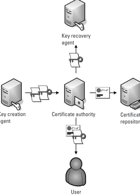
In implementations of a traditional public-key system that uses digital certificates to manage public keys, a public-private key pair is generated randomly by either a user, or an agent working on behalf of a user, in which the public key contains all of the parameters needed for using it in cryptographic calculations. Random generation of keys is not strictly required by the public-key algorithms that are used in such systems, but is required by the existing standards that define the use of such algorithms. After it is created, the public key, along with the identity of the owner of the key, is digitally signed by a certificate authority (CA) to create a digital certificate that is then used to transport and manage the key. The owner of the private key then receives a copy of the certificate and a copy of the certificate is stored in a certificate repository that is accessible by others who might need to get a user’s key. In applications where it may be necessary to recover private keys that are lost or unavailable in some way, the private keys are also securely archived by a key recovery agent. If an agent created the private key on behalf of a user, like often happens when keys are centrally generated so that copies can be archived to allow the recovery of lost or otherwise unavailable keys, the owner of the key also receives the private key from the CA. This is shown in Figure 1.1.
User Key creation
agent
Key recovery agent
Certificate authority Certificate repository
Figure 1.1 Generation of keys in a traditional public-key system.
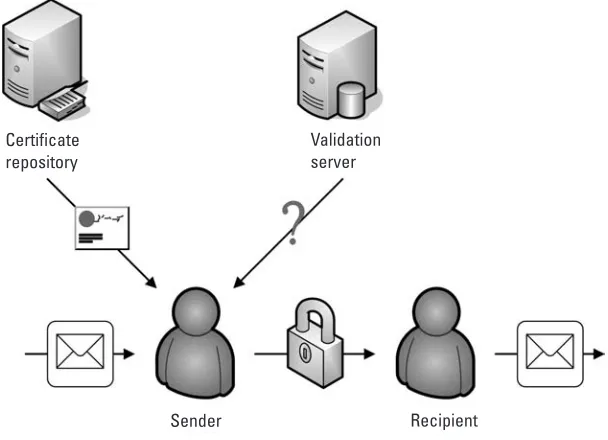
keys are needed to securely transport the 256-bit AES keys that are used today. Because generating keys and verifying users’ identities can be expensive, digital certificates are often issued with fairly long validity periods, often between one and three years. Because of the relatively long validity period of the public keys managed by digital certificates, it is often necessary to check the key in a certificate for validity before using it. This is shown in Figure 1.2. There have been many solutions proposed for validating public keys, but the existing technologies to do this are still relatively unproven and have practical difficulties when used for a large number of users.
Sender Recipient Certificate
repository
Validation server
Figure 1.2 Validation and use of a public key in a traditional public-key system.
validity status of a certificate. After any necessary validity checking is done, the user then uses the public key to encrypt information to the owner of the public key. Because the recipient has the private key that corresponds to the public key, he is able to decrypt this information. This is shown in Figure 1.2.
IBE was first mentioned by Adi Shamir in 1984 [1], when he described a rough outline of the properties that such a system should have and how it could be used, although he was unable to find a secure and feasible technology that worked as he described. He seemed to see the advantages of IBE to be related to its ease of use relative to other technologies when he described IBE in this way:
An identity-based scheme resembles an ideal mail system: If you know somebody’s name and address you can send him messages that only he can read, and you can verify the signatures that only he could have produced. It makes the cryptographic aspects of the communication almost transparent to the user, and it can be used effectively even by laymen who know nothing about keys or protocols.
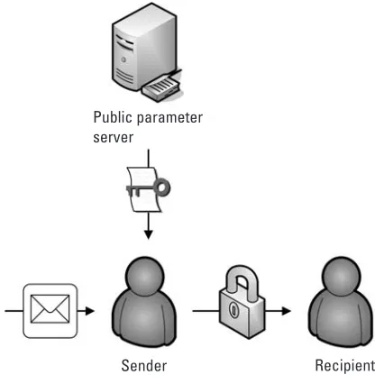
needs to get a set of public parameters from a trusted third party. With these parameters, a user can then calculate the IBE pubic key of any user and use it to encrypt information to that user. This process is shown in Figure 1.3.
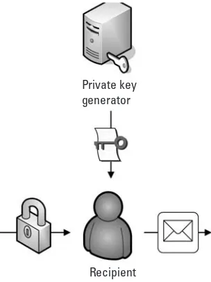
The recipient of IBE-encrypted information then authenticates in some way to a private key generator (PKG), a trusted third party that calculates the IBE private key that corresponds to a particular IBE public key. The PKG typically uses secret information called amaster secret, plus the user’s identity, to calculate such a private key. After this private key is calculated, it is securely distributed to the authorized user. This is shown in Figure 1.4. These differences are summarized in Table 1.1.
In a traditional public-key scheme, we can summarize the algorithms involved in the creation and use of a public-private key pair as key generation, encryption, and decryption. Two additional algorithms, certification and key validation, are often used in many implementations of such schemes. To fully specify the operation of such a scheme we need to define the operation of each of these algorithms. In the key generation step, one key of the public-private key pair is generated randomly and the other key in the pair is calculated from it. After this, the public key and the identity of its owner is digitally signed by a CA to create a digital certificate. Encryption is performed using the public key contained in this certificate. Decryption is performed using the private key that corresponds to the public key.
In an IBE scheme there are also four algorithms that are used to create and use a public-private key pair. These are traditionally called setup, extraction,
Public parameter server
Sender Recipient
Recipient Private key generator
Figure 1.4 Decrypting with an IBE system.
Table 1.1
Comparison of Properties of IBE and Traditional Public-Key Systems
IBE Traditional Public-Key Systems
Public parameters are distributed by a All required parameters are part of a
TTP public key
PKG master secret is used to calculate CA private key is used to create digital
private keys certificates
Private keys generated by PKG Private keys are generated randomly Public keys can be calculated by any Public keys calculated from private keys
user and transported in a digital certificate
Keys typically short-lived Keys typically valid for long periods Only encryption Digital signatures plus encryption
key of the PKG. These steps are summarized in Table 1.2. The discussions of IBE schemes in the subsequent chapters will describe the operation of IBE schemes in terms of these four parts: the algorithms that implement the setup, extraction, encryption, and decryption steps.
There are five main objectives that an information security solution can meet: providing confidentiality, integrity, availability, authentication, and nonre-pudiation. Confidentiality keeps information secret from those not authorized to see it. Integrity ensures that information has not been altered by unauthorized or unknown means. Availability ensures that information is in the place required by a user at the time that the information is required and in the form that a user needs it. Authentication is the ability to verify the identity of a user. Nonrepudiation prevents the denial of previous commitments or actions. The use of cryptography can support most of these objectives; the use of IBE can support only one of these objectives. This is summarized in Table 1.3.
Encryption of data is an easy way to provide confidentiality. In a well-designed system, decrypting encrypted data is infeasible to anyone not possessing the correct decryption key. Digital signatures provide solutions for the other
Table 1.2
Four Algorithms Comprising an IBE Scheme
Step Summary
Setup Initialize all system parameters.
Extraction Calculate IBE private key from PKG master secret and an identity using system parameters.
Encrypt Encrypt information using an IBE public key calculated from system parameters and an identity.
Decrypt Decrypt information using an IBE private key calculated from PKG master secret and an identity.
Table 1.3
Applicability of Different Encryption Technologies in Attaining Information Security Goals
Security Goal IBE Traditional Public-Key Technologies
Confidentiality Yes Yes
Integrity No Yes
Availability No Yes
Authentication No Yes
objectives of information security. They provide a way to provide integrity, because modifying digitally signed data while keeping the signature valid is as computationally infeasible as defeating the underlying cryptography that is used to create the signature. They can also provide a technical basis for nonrepudiation, although defining exactly what nonrepudiation means is fairly difficult. Not all written signatures are legally binding, after all, and we should expect the same limitations to the nonrepudiation provided by digital signatures. For all practical purposes, nonrepudiation seems to be an unattainable goal for existing informa-tion security technologies. Digital signatures also provide a way to authenticate users; a user creating a valid digital signature needs to either have possession of the private key used to create the signature or to have defeated the cryptography used to create the signature. So using digital signatures to authenticate users can also help prevent denial-of-service attacks, which increases the availability of data.
IBE provides an easy solution that provides for the confidentiality of data. It does not provide integrity, availability, authentication, and nonrepudiation. These are more easily provided by digital signatures using keys that are created and managed by a traditional public-key system. As we will see, however, the advantages that IBE provides make it a very good solution for some problems, and a hybrid solution that used IBE for encryption and a traditional public-key system to provide digital signatures may be a solution that combines the best features of each technology.
1.2 Why Should I Care About IBE?
IBE is an interesting technology because other public-key algorithms have encountered practical difficulties in use. In particular, implementations of tradi-tional public-key technologies have gained a reputation for being difficult and expensive, at least when they are used by people; the most successful application of public-key technology has been in the widespread use of SSL, which requires minimal interaction with a user when it is used to authenticate a server and to encrypt communications with the same server. Applications that require a user to mange or use public keys have not been as successful.
technol-ogy, and has probably been one of the major factors hindering the widespread adoption of public-key technology. Dan Geer even conjectured that high costs are unavoidable when using any type of cryptography [4]:
Both symmetric cryptosystems, like Kerberos, and asymmetric cryptosys-tems, like RSA, do the same thing—that is to say they do key distribution— but the semantics are quite different. The fundamental security-enabling activity of a secret key system is to issue fresh keys at low latency and on demand. The fundamental security-enabling activity of an asymmetric key system is to verify the as-yet-unrevoked status of a key already in circulation, again with low latency and on demand. This is key management and it is a systems cost; a secret key system like Kerberos has incurred nearly all its costs by the moment of key issuance. By contrast, a public key system incurs nearly all its costs with respect to key revocation. Hence, a rule of thumb: The cost of key issuance plus the cost of key revocation is a constant, just yet another version of ‘‘You can pay me now or you can pay me later.
Geer’s conjecture tells us that we should expect any use of cryptography to be expensive. Because there are many cases where the use of encryption is desirable, a new type of encryption technology that avoids some of the problems associated with traditional public-key technologies is inherently interesting, and this is one of the promises of IBE. IBE may not offer any new capabilities that traditional public-key technologies cannot provide, but it allows for the creation of solutions that would be very difficult and expensive to implement with earlier technologies. In particular, these solutions seem to violate Geer’s principle that using encryption has to have a high cost.
Key validation, or checking to make sure that a particular key is valid at some point in its lifetime, can be an expensive and difficult process, particularly when validating uses of a key that took place in the past. Suppose that you are doing digitally signed and encrypted electronic transactions and you need to verify whether or not a particular transaction had a valid signature at some point in the past, like when the transaction took place two years ago. The validity of a digital certificate can change during its lifetime as it is temporarily suspended or revoked, so it is necessary to be able to reconstruct the validity of the key managed by any certificate at any point in the key’s lifetime to be able to answer such questions. Doing so requires being able to reconstruct the state of the system that manages the validity of keys, which is a complex and difficult problem.
precision as the ability to immediately revoke or suspend a key, but it makes the validation of such keys trivial. This, in turn, lets us build simpler and less expensive systems. The ability to quickly and easily calculate keys makes short-lived keys in IBE practical, where they are often impractical, although not impossible, to use in a system based on traditional PKI technology.
Key recovery, the capability to restore a lost or otherwise-unavailable key, is an essential feature for commercially successful encryption technology. In practice, most key recovery is apparently performed when passwords protecting access to keys are lost or forgotten [5] instead of the scenario in which the owner of a key is not present, yet there is an immediate need for information encrypted with his key. In traditional public-key systems, key recovery is typically implemented through having a TTP generate keys on behalf of a user and securely archiving a copy of the user’s private key that can be used for key recovery as needed. Such key recovery systems require securely storing archival copies of all private keys and carefully controlling access to the archive of these keys.
IBE systems, on the other hand, calculate keys as needed, so there is no need for archiving keys at all. The only information that needs to be backed-up is the master secret that is used by the PKG to calculate IBE private keys. This simpler process makes IBE systems simpler and easier in many applications than traditional public-key technologies, and can make the cost of supporting and maintaining an IBE system much less than the cost of supporting and maintaining a system with the same capabilities that is based on traditional public-key technology. It also provides IBE systems with some capabilities that can be fairly difficult to implement with traditional public-key technologies.
The ability to calculate public and private keys as needed is a subtle difference between IBE and traditional public-key technologies, but one that provides many useful properties. In particular, it is not necessary to enroll a user before encrypting information to them. Therefore, it is easy to IBE-encrypt information to a user that does not exist yet and rely on the future user to properly authenticate before he can decrypt the information. If a validity period is part of an identity, it is possible to encrypt information that can only be decrypted at some point in the future, for example. Or, in a response to a natural disaster, responders may want to securely communicate with other responders, but they may not know with whom they will need to communicate before a disaster happens. Because it is impractical to pre-enroll every potential responder to every type of disaster, a technology that allows encrypting informa-tion to users before they are enrolled can be useful in circumstances like this. IBE provides a useful way to accomplish this.
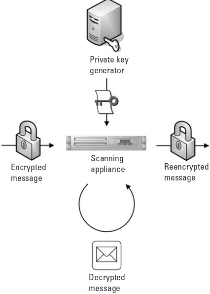
efforts to acquire sensitive personal information, bank account numbers or credit card numbers. To combat this growing threat, many organizations implement filtering on both incoming and outgoing e-mail messages to protect users from such malicious messages. Organizations may also want to search outgoing mes-sages for sensitive information and process it in some way that ensures that no sensitive material is sent unencrypted over a public network. Some organizations return the original message to the sender with a warning to encrypt such sensitive content in the future. Others want to automatically encrypt such messages. Using IBE, it is not difficult to scan even encrypted messages for unsuitable content. Delegate the authority to retrieve IBE private keys to a scanning process, and the scanning process can then request IBE keys on behalf of the owner of the private key, scan the decrypted message for unsuitable content, and reencrypt the message after it is scanned by using the recipient’s IBE public key that it can easily calculate. This is shown below in Figure 1.5. It is possible to implement a similar solution using traditional public-key technologies, but it is typically much more complex and difficult to implement.
Decrypted message
Scanning appliance Encrypted
message
Reencrypted message Private key
generator
Existing information security architectures focus on creating and main-taining a security perimeter. Inside the perimeter it is supposed to be relatively secure, and the perimeter is designed to keep threats away from the protected network. Trends in both the organization of businesses and the evolution of technology have made this model more and more difficult to implement.
One trend in the organization of businesses is the continuing integration of business partners to help all of the participants gain from the lower costs of tightly integrated operations. In the case of credit card processing, for example, the networks of the merchants who accept credit cards, the banks that issue credit cards, and the credit card companies themselves are now tightly integrated to make the processing of credit card transactions more efficient. In situations like this, it can sometimes be difficult to determine exactly where the network perimeter is, which makes it very difficult to create and maintain a security architecture that relies on a strong security perimeter.
Wireless devices also broadcast data without regard for a logical security perimeter, and thus make it difficult to implement security that is based on enforcing such a perimeter because an eavesdropper can easily intercept wireless transmissions without having to physically connect to a network. Situations like these are leading to an alternative to a highly secure perimeter: a security architecture in which we protect the data that resides in the network instead of the network itself.
One way to implement a security architecture in which we protect data instead of the network is by using encryption, where we encrypt data so that only the authorized users can decrypt it. IBE can use any arbitrary data for an identity, including strings encoding roles. So it is possible to use IBE to encrypt sensitive medical records using ‘‘doctor’’ as part of an identity, for example, and then to require users to prove that they are authorized to access such data when they request the IBE private key needed to decrypt it.
IBE may make it particularly useful to solve the problems that this different model of security will present.
So it appears that the properties of IBE give systems that use the technology interesting properties and allow for the creation of solutions that may be easier to use and less expensive to support than solutions provided by traditional public-key technologies. On the other hand, IBE only provides the capability to encrypt and does not allow the creation of digital signatures. This means that a complete information security solution using IBE, one that provides confidentiality, integrity, availability, authentication, and nonrepudiation, may need to be a hybrid solution that uses both IBE and traditional public-key technologies to provide a solution that takes advantage of the strengths of each of the technologies. Such solutions may eventually reduce the cost of using encryption to the point where it will be used on a wide scale, violating Geer’s principle that any use of encryption must be expensive. The promise of such solutions is what motivated the existing commercial applications of IBE and will probably also motivate future applications of the technology.
References
[1] Shamir, A., ‘‘Identity-Based Cryptosystems and Signature Schemes,’’ Proceedings of CRYPTO ’84, Santa Barbara, CA, August 19–22, 1984, pp. 47–53.
[2] Whitten, A., and J. Tygar, ‘‘Why Johnny Can’t Encrypt: A Usability Evaluation of PGP 5.0,’’Proceedings of the 8th USENIX Security Symposium, Washington, D.C., August 23–26, 1999, pp. 169–184.
[3] Sheng, S., et al., ‘‘Why Johnny Still Can’t Encrypt: Evaluating the Usability of Email Encryption Software,’’Proceedings of the 2006 Symposium on Usable Privacy and Security, Pittsburgh, PA, July 12–14, 2006.
[4] Geer, D., ‘‘Risk Management Is Where the Money Is,’’Risks Digest, Vol. 20, No. 6, 1998, pp. 1–9.
2
Basic Mathematical Concepts and
Properties
This chapter contains a review of all of the necessary definitions needed in the following chapters in which we discuss IBE algorithms. It also provides a list of the notation that we will use in the following chapters and states without any proofs various facts that will be cited in following chapters. Proofs of the facts listed in this chapter maybe found in [1, 2].
2.1 Concepts from Number Theory
Number theory concerns the properties of the integers and their generalizations, and provides a foundation for the other concepts that follow in later sections. The set of natural numbers {1, 2, 3, . . .} is denoted by the symbol ⺞.
The set of integers {. . ., −3, −2, −1, 0, 1, 2, 3, . . .} is denoted by the symbol⺪.
The set of real numbers is denoted by the symbol ⺢.
The set of complex numbers is denoted by the symbol ⺓. Elements of⺓
can be written asa +bi, where a andbare real numbers andi2 = −1. Definition If a and bare integers, then a divides b or a is a divisor ofb if there exists an integercsuch that b=ac. In this case we write a| band we say thata is afactorof b.
Example 2.1
(i) Note that 1,001=7⭈ 11⭈ 13, so that 7| 1,001 and 7 is a factor of 1,001.
(iii) We can also write 1,001=(−7)⭈ (−11)⭈ 13, so−7 and−11 are also factors of 1,001.
Definition 2.1
An integerp ≥ 2 is aprime if its only positive divisors are 1 and p.
Definition 2.2
A primepis a Solinas prime if we can writep =2a ±2b± 1 for some positive integers a and b. Such primes are useful in the efficient implementation of many IBE algorithms, in which we need to perform a double-and-add iteration on the binary expansion of a prime. If we use a Solinas prime in such algorithms, the low density of a Solinas prime of the form p = 2a + 2b + 1 will clearly minimize the number of operations needed to implement such an iteration. The cases wherep=2a±2b±1 can be similarly implemented very efficiently by representing p in nonadjacent form [3]. In the following we will always assume that a Solinas prime is of the formp =2a + 2b+ 1.
Example 2.2
(i) The prime 41= 25 +23+ 1 is a Solinas prime. (ii) The prime 29= 25 −22+ 1 is a Solinas prime.
Definition 2.3
LetF={p1,p2, . . . ,pn} be a set of primes. We say an integernis F-smooth is all of the prime factors ofn are elements ofF.
Definition 2.4
A nonnegative integerd is thegreatest common divisor of integers aandb ifd is the largest positive integer that divides both a and b. This is denoted by d=gcd (a,b).
Example 2.3
(i) If a = 1,001 = 7 ⭈ 11 ⭈ 13 and b = −286 = −2 ⭈ 11 ⭈ 13, then gcd (a,b)= 11 ⭈ 13 =143.
(ii) If a =11 andb =13, then gcd (a,b) =1.
2.1.1 Computing the GCD
to gcd (a, b), this algorithm also returns integers x and ysuch that gcd (a, b)
=ax +by.
Algorithm 2.1: extended_gcd INPUT: integersa, bwitha ≥ b
OUTPUT: gcd (a,b), integersx andysuch that gcd (a,b) =ax +by
1. If b=0
2. d← a, x← 1, y← 0, return (d,x, y) 3. x1← 0, x2← 1, y1← 1, y2 ←0 4. While b>0
5. q← a/b, r← a −qb, x← x2 −qx1, y ←y2 −qy1 6. a ← b, b← r, x2 ← x1,x1 ←x, y2 ← y1,y1 ← y 7. d← a, x← x2,y ← y2, return (d, x, y)
Definition 2.5
For integersaandb, if gcd (a,b) then we say thataandbarerelatively prime.
Example 2.4
(i) If a = 1,001 andb =286, then gcd (a, b) = 77, so a andbare not relatively prime.
(ii) If a = 11 andb =13, then gcd (a, b) =1, so a and bare relatively prime.
Definition 2.6
If a, b, and n are integers, then we say thata is congruent to b modulo nif n divides (b −a) and we write a≡ b(modn).
Example 2.5
(i) 7 ≡3(mod 4) because 4 | (7 −3). (ii) 11≡ 3(mod 4) because 4| (11− 3). (iii) −7 ≡2(mod 3) because 3 | (−7 −2). (iv) 7 ≡11(mod 4) because 4 | (7 −11).
Property 2.1 (Chinese Remainder Theorem)
x ≡a1 (modn1)
x ≡a2 (modn2) ⯗
x ≡ak (modnk)
Property 2.2 (Gauss’ Algorithm)
The solution to the system of congruences given in Property 2.1 can be computed as
x=
∑
k
i=1
aiNiMi mod n (2.1)
where
Ni = nn i
and
Mi =Ni−1 modni
Gauss’ algorithm can be written in a slightly different way that makes it easier to understand. In particular, note that we can also write (2.1) as
x=
∑
k
i=1
ai ⭈ ei mod n
where each ei has the property that
ei ≡
再
1 (mod ni) 0 (mod nj), j ≠iSo we can think of Gauss’ algorithm as being essentially an integer version of Lagrange interpolation, where we fit a polynomial tok points by creating a similar set of coefficients that are either 0 or 1 and thus force the desired behavior at the given points.
Example 2.6
Consider the following system of congruences:
x ≡2 (mod 3) = a1(modn1)
Applying Gauss’ algorithm, we find that
n= n1n2 =3 ⭈ 4 =12
N1 = n n1
=12
3 = 4
N2 =
n n2
=12
4 = 3
M1 =N1−1 modn1 = 4−1 mod 3= 1 M2 =N2−1 modn2 = 3−1 mod 4= 3
so that
x =(a1N1M1 + a2N2M2) mod 12 =(2 ⭈ 4 ⭈ 1 +3 ⭈ 3 ⭈ 3) mod 12
=(2 ⭈ 4 +3 ⭈ 9) mod 12
=(8 + 27) mod 12 =35 mod 12 =11 mod 12
In this example we can also think of Gauss’ algorithm as finding integers e1 ande2such that we have
x =(2 ⭈ e1 +3 ⭈ e2) mod 12
Gauss’ algorithm then finds e1= 4 and e2 = 9, where we have
e1 = 4≡
再
1 (mod 3) 0 (mod 4)
and
e2 = 9≡
再
0 (mod 3) 1 (mod 4)
Definition 2.7
Property 2.3
Ifm andn are relatively prime then(mn) = (m)(n).
Example 2.7
(i) (7)=6 because each of the integers 1, 2, 3, 4, 5, and 6 are relatively prime to 7.
(ii) (p) = p − 1 for any prime p because 1, 2, 3, . . . , p − 1 are all relatively prime to p.
(iii) (77)= (7)(11)= 6 ⭈ 10 =60.
Property 2.4 (Fermat’s Little Theorem)
Letp be a prime anda be any integer. Then we have that
ap≡ a(modp)
Ifa is relatively prime to p, then we also have that
ap−1≡ 1 (mod p)
Example 2.8
(i) For p =5 and a = 2, we have thatap= 25 =32 ≡ 2(mod 5). (ii) For p =5 and a = 2, we have thatap−124= 16 ≡1(mod 5). (iii) For p = 5 and a = 10, we have that ap = 105 = 100,000 ≡
0(mod 5)≡ 10(mod 5).
(iv) For p = 5 and a = 10, we have that ap−1 24 = 10,000 ≡ 0(mod 5)≡/ 1(mod 5).
Property 2.5 (Euler’s theorem)
Letn be an integer and a be an integer relatively prime to n. Then we have that
a(n)≡ 1 (mod n)
Example 2.9
(ii) Withn=5⭈ 7, we have that(n)=24 and that 524≡1(mod 35). (iii) Withn = 11 ⭈ 13 = 143, we have that (n) = 120 and that 11120
≡ 1(mod 143).
Definition 2.8
We use⺪n to denote the set of integers {0, 1, . . ., n− 1}.
We can perform arithmetic on elements of ⺪
n by reducing a sum or
product to the remainder that is left after dividing byn, which we callreducing modulo n. In ⺪n we havea + b = cwhen (a +b) ≡ c(mod n). Even though
we define ⺪n to only include the integers from 0 through n − 1, it is often
convenient to think of n − 1 as being −1, even though −1 is not really an element of ⺪
n.
Example 2.10
(i) In ⺪12 we have that 9+ 6= 3, or 9+ 6 ≡3(mod 12).
(ii) In ⺪9we have that 3 ⭈ 3 =0, or 3 ⭈ 3≡ 0(mod 9).
As Table 2.1 shows, not every element of ⺪5 has a square root in⺪5. In
particular, 0, 1, and 4 have square roots in ⺪5 while 2 and 3 do not. This
motivates the following definitions.
Definition 2.9
A nonzero elementa∈⺪nis called aquadratic residuemodulonif there exists
somex∈⺪nwithx2≡a(modn). If no suchxexists, we say thatais aquadratic
nonresiduemodulon.
Example 2.11
(i) From Table 2.1 we see that 0, 1, and 4 are quadratic residues modulo 5.
(ii) From Table 2.1 we see that 2 and 3 are quadratic nonresidues modulo 5.
Table 2.1 Multiplication in⺪5
* 0 1 2 3 4
0 0 0 0 0 0
1 0 1 2 3 4
2 0 2 4 1 3
3 0 3 1 4 2
Legendre symbols are a notation that indicates whether or not an integer is a quadratic residue.
Definition 2.10
Letp be an odd prime and a an integer. Then the Legendre symbol
冉
a p冊
is defined to be(i) 0 ifp divides a.
(ii) +1 ifa is a quadratic residue modulo p. (iii) −1 ifa is a quadratic nonresidue modulo p.
Property 2.6
Leta and b be integers and p and qbe odd primes. Then Legendre symbols have the following properties:
Property 2.6(i) tells us that −1 is a quadratic residue modulo p if p ≡
1(mod 4) and that−1 is a quadratic nonresidue modulop ifp ≡3(mod 4). If
−1 is a quadratic nonresidue modulop, then we have that
冉
−aso that eitherais a quadratic residue or−ais a quadratic residue. In particular, this is true whenp ≡3(mod 4).
冉
p(iii) Because 3 and 7 are both congruent to 3 modulo 4, we have that
冉
73
冊
= −冉
3 7冊
= +1We can generalize the definition of Legendre symbols to get Jacobi symbols, which are defined for composite denominators as follows.
Definition 2.11
Leta be an integer andn be a positive odd integer with
n=
写
is a Legendre symbol as defined in Definition 2.10.
Property 2.7
(i)
冉
aresidue modulo n if and only if a is a quadratic residue modulo p and a is a quadratic residue modulop.
2.1.2 Computing Jacobi Symbols
冉
aThis gives us the following algorithm for computing Jacobi symbols. Note that it is not necessary to know the factorization ofn to do this.
Algorithm 2.2: JacobiSymbol
INPUT: odd integern ≥3, integer a with 0 ≤ a< n OUTPUT: Jacobi symbol (a/n)
1. Ifa =0, return 0
Abstract algebra provides the framework for defining the differences and similari-ties between different algebraic structures. The real numbers and the integers are fundamentally alike in some ways and different in other ways, for example, and the framework of abstract algebra provides a way to describe these properties and generalize them to other structures. In particular, structures that are suitable for use in computers have finite-length representations, so we want to understand the properties of structures that behave much like the real numbers yet are finite instead of infinite.
Definition 2.12
Definition 2.13
Agroup(G, *) is a setGand a binary operation * onGthat has the following properties:
(i) a * (b* c) =(a * b) *cfor all a, b,cin G(associativity).
(ii) There is a special element ofGcalled theidentity element which we write as e. This identity element satisfies a* e =e* a = a for all a inG.
(iii) Each element a of G has an inverse that we write as a−1, also an element of G, such thataa−1 =a−1a = e.
We say that Gis a group under the operation * if (G, *) is a group. We will also somewhat inaccurately say that a set Gis a group without listing the group operation if the operation is clear from the context of the discussion, so we might say that ‘‘the integers are a group,’’ for example, even though it is somewhat inaccurate.
Example 2.14
(i) The integers ⺪ under addition are a group. In this case, the integer
0 acts as the identity element.
(ii) The integers⺪ under multiplication are not a group because not all
integers have multiplicative inverses that are also in⺪. The
multiplica-tive inverse of 3 is not an integer, for example.
(iii) The natural numbers⺞under addition are not a group because the
natural numbers lack an additive identity, that is, 0 ∈⺞.
(iv) The nonzero real numbers under multiplication form a group. In this case, the real number 1 acts as the identity element.
(v) ⺪nis a group under addition but may not be a group under
multiplica-tion; ⺪nis a group under multiplication if and only if nis prime.
(vi) The set V = {0, 1, 2, 3} along with the operation shown in Table 2.2 is a group. In this group, every element is its own inverse.
Definition 2.14
If (G, *) is a group, then the number of elements in the set G is called the orderof the group. This can be either finite or infinite.
Definition 2.15
Table 2.2 Operations in the GroupV
* 0 1 2 3
0 0 1 2 3
1 1 0 3 2
2 2 3 0 1
3 3 2 1 0
Example 2.15
(i) The integers under addition are an Abelian group.
(ii) The set of all 2 × 2 invertible matrices with real entries is a group under matrix multiplication, but not an Abelian group because matrix multiplication is not commutative.
If a group is Abelian we often write the group operation as +instead of * and using+to denote a group operation is usually reserved for Abelian groups. Writing a * b ≠ b * a is fine, because not all groups are Abelian, but if you writea + b≠b+ a it will make many mathematicians uncomfortable.
Definition 2.16
If (H, *) and (G, *) are groups and H is a subset of G, then we say H is a subgroup of G. Note that this means that the subgroup must have the group structure with respect to the same operation that defines the group structure inG.
Example 2.16
(i) The even integers under addition are a subgroup of the integers under addition.
(ii) The odd integers under addition are not a subgroup of the integers under addition.
(iii) The groupV={0, 1, 2, 3} of Example 2.14(vi) has three subgroups of order 2: H1 ={0, 1},H2= {0, 2}, andH3 = {0, 3}.
Definition 2.17
Let (G, *) be a group with identity elementeandg∈G. The smallest positive integern such that
g * g * . . . * g =gn =e 1442443
is called theorder of the element g. If no such integer exists then we say that the order of gis infinite.
Example 2.17
(i) In the group (⺪7,+) the order of the element 2 is 7.
(ii) In the group (⺪6,+) the order of the element 2 is 3.
(iii) In the group (⺪,+) the order of the element 1 is infinite.
Property 2.9 (Lagrange’s theorem)
The order of any element of a group divides the order of the group.
Property 2.10
LetGbe a group of order n andp a prime. If p
|
n butp2⁄
|
n, then G has a unique subgroup of orderp. In some IBE systems we need to map an identity to a point of prime order, and knowing that this mapping will map the identity to an element of a particular subgroup is useful.Example 2.18
(i) The group⺪132has order 132=22⭈ 3 ⭈11 and thus has a unique
subgroup of order 11. Given any element of g ∈⺪132, we can find
an element of the subgroup of order 11 by calculating
冉
13211
冊
g =12 ⭈ g(ii) The groupVof Example 2.14(vi) is of order 4 but has three different subgroups of order 2.
Definition 2.18
A group (G, *) is cyclic if there exists a g ∈G such that for anyh ∈Gthere exists an integerisuch that we can writeh=gi. Such an elementgis called a generatorofGand we write G= 〈g〉 to indicate this.
Example 2.19
(i) If pis a prime, then any nonzero element of⺪
pgenerates the group
⺪pand the group ⺪pis cyclic.
(ii) Both 1 and 5 generate ⺪6, while 2, 3, 4 do not generate⺪6.
Definition 2.19
Definition 2.20
Let G be a group generated by g. For any a ∈G, we say that the discrete logarithmto the basegofais␣if we have that␣is the smallest positive integer such that a= g␣.
Example 2.20
(i) In the groupG= (⺪
n, +), we have thatG= 〈1〉, and that the discrete
logarithm of k =k ⭈ 1 to the base 1 is k.
(ii) In the groupG=(⺪11* ,×), we have thatG= 〈2〉, and that the discrete
logarithm of 6 ≡29(mod 11) to the base 2 is 9.
In some cases, we will have two groups that behave exactly the same way, but are labeled differently in some way. In a trivial case, we could write one version of the integers in an italic font and another version in bold font and notice that these two versions behave exactly the same way if we ignore this slight difference. So while we could not add an italic 2 to a bold font 2, for example, we can easily map the two sets to each other by making the necessary font change. The desire to find a way to define how two structures have the same properties but with changed names motivates the following definition.
Definition 2.21
Let f be a function from a group (G, +) to a group (H, ⊕). Then f is a homomorphismof groups if we have thatf(a +b) =f(a) ⊕f(b) for alla and bin G. A homomorphism of groups is a function that preserves some of the structure of a group but not necessarily all of the structure.
Definition 2.22
Letf be a homomorphism from a group (G, +) to a group (H,⊕). Then f is anisomorphism of groups if it has the following properties:
(i) For every a andbin G, iff(a) =f(b) then a = b. (ii) For each h∈H there exists a g ∈Gwithh= f(g).
When these properties hold, we say that the groups (G, +) and (H, ⊕) areisomorphicand writeG≅H to indicate this. An isomorphism is a function that preserves all of the structure of a group, and groups that are isomorphic are essentially identical, differing only in the way that their elements are written.
Definition 2.23
Example 2.21
(i) Ifeis the identity element of a group (G,+), then the functionf(g)
=efor anyg∈Gis a homomorphism of groups, where the range of f implicitly lies in the trivial group containing just the element e. This is not an isomorphism because it fails property (i) of Definition 2.20.
(ii) The mappingfwheref(n)=2nis a group homomorphism from the integers under addition to the even integers under addition because f(a +b)= 2 (a + b) =2a + 2b= f(a)+ f(b). This mapping falso satisfies properties (i) and (ii) of Definition 2.22, so it is also an isomorphism.
(iii) The real numbers under addition are isomorphic to the positive real numbers under multiplication, with an isomorphism given by f(x) = ex.
(iv) Complex conjugation, that is,f(a+bi)=a−bi, is an endomorphism of the complex numbers under addition.
Definition 2.24
Afield (F,+, *) is a setFand a two binary operations+ and * onFthat have the following properties for alla, b, cinF.
(i) (F, +) is an Abelian group.
(ii) Let F* denote the set of elements of F not equal to the identity element for the operation +. Then (F*, *) is an Abelian group. We think of F* as being the nonzero elements ofF.
(iii) a * (b+ c) = a* b +a * c(distributivity).
Note that only two operations are defined in a field, which we think of as addition and multiplication. Subtraction and division are not defined, so when (F,+, *) is a field and a andb are elements ofF, when we write a −b we really mean a + (−b) where −b is the inverse of bunder the operation + and when we writea/bwe really meanab−1whereb−1is the inverse ofbunder the operation *.
Example 2.22
(i) (⺢, + ⭈) is a field. Property (ii) of Definition 2.24 tells us that all
(ii) If p is a prime, (⺪p, +, ⭈) is a field.
(iii) The set of polynomials with real coefficients with the operations of addition and multiplication of polynomials is a field.
(iv) The set of all polynomials with real coefficients with addition and multiplication performed modulo the polynomial x2+ 1 is a field. (v) If p is a prime, the set of all polynomials with coefficients from ⺪p
with the operations of polynomial addition and multiplication is a field.
As with groups, we will somewhat inaccurately say that the setFis a field without listing the field operations if the operations are clear from the context of the discussion.
Definition 2.25
If (F, +, *) is a field, then the number of elements in the set F is called the order of the field. This can be infinite or finite. We write ⺖
qfor a finite field
withqelements.
Definition 2.26
If (F, +, *) is a field and nis the smallest positive integer such that
x+ x+ . . . +x =nx =0 1442443
n times
for all x ∈F is called the characteristic of the field. If no such integer exists, then we say that the field hascharacteristic zero.
Example 2.23
(i) If p is a prime, then the field⺖
phas characteristicp.
(ii) The field of real numbers has characteristic zero.
(iii) Ifp is a prime, the field of polynomials with coefficients from⺖p is
a field of characteristic p. This field is infinite, yet has character-istic p.
Definition 2.27
Ahomomorphism of fields is function that preserves some of the structure of a field. Letf be a function from a field (K,+, *) to a field (F,⊕, ⊗). Then fis ahomomorphism of fields if we have that
and
f(a * b) =f(a) ⊗f(b)
for all aandb inK.
Definition 2.28
An isomorphism of fields is a function that preserves all of the structure of a field. Let f be a homomorphism from a field (K, +, *) to a field (F, ⊕, ⊗). Then fis an isomorphism of fields if it has the following properties:
(i) For every a andbin K, iff(a) =f(b) then a =b. (ii) For each b∈Fthere exists a a ∈K withb= f(a).
When these properties hold, we say that the fields (K, +, *) and
(F,⊕,⊗) are isomorphicand write K ≅F to indicate this. An isomorphism is a function that preserves all of the structure of a field, and fields that are isomorphic are essentially identical, differing only in the way that their elements are written.
Example 2.24
The field of complex numbers is isomorphic to the field of polynomial with real coefficients modulo the polynomialx2+1, and we can write an isomorphism fbetween the two fields explicitly as f(a+ bi) =a + bx.
Property 2.11
Any field with a finite number of elements has a number of elements equal to pnfor some primepand some natural numbern. All finite fields with the same number of elements are isomorphic, so we can talk about the finite field ⺖
q,
even if there may be different ways to represent the elements of this field.
Definition 2.29
If (K, +, *) and (F, +, *) are fields andK is a subset of F, then we sayK is a subfield of F. Note that this means that the subfield K has to have the field structure with respect to the same operations that defines the field structure in F.
Definition 2.30
IfK is a subfield of a field F, then we say that Fis an extension fieldof K.
Example 2.25
(ii) The field ⺖q is not a subfield of the real numbers. Although the
elements of ⺖
q are a subset of the real numbers ifq is a prime, the
operations defined on⺖qare different from those defined in the real
numbers, so ⺖
qcannot be a subfield of the real numbers. In⺖3, for
example, we have that 2+2=1, which is different than the fact that 2+2=4 in the real numbers. A more careful description of⺖3might
write its elements as 0ˆ, 1ˆ, and 2ˆ and its operation as⊕to make this explicit.
Definition 2.31
IfFis an extension field of K, thenFis a vector space of dimension kover K for some positive integerk. The value ofkis called thedegreeof the extension. The degree of an extension may be either finite or infinite. If k is finite then we can write a typical element of F as ␣ =(x1, x2, . . . ,xk) where each
xi ∈K.
Example 2.26
(i) The complex numbers are an extension field of degree 2 of the real numbers and we can write a complex number z = x + iy as z=(x,y) to emphasize the fact that complex numbers can be consid-ered vectors with real coordinates.
(ii) Polynomials with real coefficients are an extension field of infinite degree of the real numbers.
(iii) Let v ∈⺖q and ␣ be a solution to the equation xd− v= 0 with
␣n≠v forn<d. So if ␣is a sixth root ofv, for example, then it is not a cube root or square root. Then the smallest extension to⺖qin
whichxd− v= 0 has a solution is ⺖qd.
(iv) Suppose thatF3 is a finite field that is an extension of degreek2 of
the finite fieldF2and thatF2is a finite field that is an extension of
degree k1 of the finite field F1. Then by writing an element of F3
in terms of the basis ofF2and then writing the basis ofF2in terms of the basis of F1 we see thatF3 is an extension of degreek1k2 of
the finite field F1.
Suppose that if q = pn for some prime p and that ⺖q is an
group structure under the operation of addition that the definition of a field requires. Because ⺖
qis a vector space of dimensionn over
⺖p, we can talk about elements of ⺖q being linearly independent,
which has the same meaning as in linear algebra.
Definition 2.32
Elements of⺖qkxandyarelinearly independentif for alla,b∈⺖qwe have that
a⭈ x +b ⭈y = 0 implies thata =0 and b= 0.
Example 2.27
(i) In ⺖112 (0, 1) and (1, 0) are linearly independent.
(ii) In ⺖112 (0, 1) and (0, 2) are not linearly independent because (0, 1)
+ 5⭈ (0, 2) ≡(0, 0) (mod 11).
To make ⺖
q a field, however, we also need to be able to multiply such
vectors and to be able to find their multiplicative inverses. One way to do this is to identify the components of a vector with coefficients of a polynomial and then multiply vectors as if they were the polynomials created in this way. So we identify a= (a0, . . . ,an−1) with the polynomial f(x)=
a0+ a1x+ . . . +an−1xn−1. Definition 2.33
If F is a field, we write F[x] for the set of all polynomials in the variable x with coefficients fromF.
Example 2.28
(i) (3 + 2i)x2 +(1 + i)x+ 1 ∈⺓[x]
(ii) 7x2 +2x+ 1∈⺖11[x]
Definition 2.34
If F is a field and f(x) ∈F[x], then we write F[x]/(f(x)) for the set of polynomials inF[x] reduced modulo the polynomialf(x).
Example 2.29
(i) In⺢[x]/(x2 +1) we do calculations modulo the polynomialx2+1,