Introduction to Probability and Statisti (3)

(1)

Introduction to Probability

and Statistics Using

R

G. Jay Kerns

(2)

IP_S_{UR: Introduction to Probability and Statistics Using}R

Permission is granted to copy, distribute and/or modify this document under the terms of the GNU Free Documentation License, Version 1.3 or any later version published by the Free Software Foun-dation; with no Invariant Sections, no Front-Cover Texts, and no Back-Cover Texts. A copy of the license is included in the section entitled “GNU Free Documentation License”.

(3)

Preface

This book was expanded from lecture materials I use in a one semester upper-division undergradu-ate course entitledProbability and Statisticsat Youngstown State University. Those lecture mate-rials, in turn, were based on notes that I transcribed as a graduate student at Bowling Green State University. The course for which the materials were written is 50-50 Probability and Statistics, and the attendees include mathematics, engineering, and computer science majors (among others). The catalog prerequisites for the course are a full year of calculus.

The book can be subdivided into three basic parts. The first part includes the introductions and elementarydescriptive statistics; I want the students to be knee-deep in data right out of the gate. The second part is the study ofprobability, which begins at the basics of sets and the equally likely model, journeys past discrete/continuous random variables, and continues through to multivariate distributions. The chapter on sampling distributions paves the way to the third part, which is in-ferential statistics. This last part includes point and interval estimation, hypothesis testing, and finishes with introductions to selected topics in applied statistics.

I usually only have time in one semester to cover a small subset of this book. I cover the material in Chapter 2 in a class period that is supplemented by a take-home assignment for the students. I spend a lot of time on Data Description, Probability, Discrete, and Continuous Distributions. I mention selected facts from Multivariate Distributions in passing, and discuss the meaty parts of Sampling Distributions before moving right along to Estimation (which is another chapter I dwell on considerably). Hypothesis Testing goes faster after all of the previous work, and by that time the end of the semester is in sight. I normally choose one or two final chapters (sometimes three) from the remaining to survey, and regret at the end that I did not have the chance to cover more.

In an attempt to be correct I have included material in this book which I would normally not mention during the course of a standard lecture. For instance, I normally do not highlight the intricacies of measure theory or integrability conditions when speaking to the class. Moreover, I often stray from the matrix approach to multiple linear regression because many of my students have not yet been formally trained in linear algebra. That being said, it is important to me for the students to hold something in their hands which acknowledges the world of mathematics and statistics beyond the classroom, and which may be useful to them for many semesters to come. It also mirrors my own experience as a student.

The vision for this document is a more or less self contained, essentially complete, correct, introductory textbook. There should be plenty of exercises for the student, with full solutions for some, and no solutions for others (so that the instructor may assign them for grading). BySweave’s dynamic nature it is possible to write randomly generated exercises and I had planned to implement this idea already throughout the book. Alas, there are only 24 hours in a day. Look for more in future editions.

(8)

Seasoned readers will be able to detect my origins: Probability and Statistical Inference by Hogg and Tanis [44],Statistical Inferenceby Casella and Berger [13], andTheory of Point Estima-tion/Testing Statistical Hypothesesby Lehmann [59, 58]. I highly recommend each of those books to every reader of this one. SomeRbooks with “introductory” in the title that I recommend are Introductory Statistics withRby Dalgaard [19] andUsingRfor Introductory Statisticsby Verzani [87]. Surely there are many, many other good introductory books aboutR, but frankly, I have tried to steer clear of them for the past year or so to avoid any undue influence on my own writing.

I would like to make special mention of two other books: Introduction to Statistical Thought by Michael Lavine [56] andIntroduction to Probabilityby Grinstead and Snell [37]. Both of these books arefreeand are what ultimately convinced me to release IP_S_URunder a free license, too.

Please bear in mind that the title of this book is “Introduction to Probability and Statistics UsingR”, and not “Introduction to R Using Probability and Statistics”, nor even “Introduction to Probability and Statistics and R Using Words”. The people at the party are Probability and Statistics; the handshake isR. There are several important topics aboutRwhich some individuals will feel are underdeveloped, glossed over, or wantonly omitted. Some will feel the same way about the probabilistic and/or statistical content. Still others will just want to learnRand skip all of the mathematics.

Despite any misgivings: here it is, warts and all. I humbly invite said individuals to take this book, with the GNU Free Documentation License (GNU-FDL) in hand, and make it better. In that spirit there are at least a few ways in my view in which this book could be improved.

Better data. The data analyzed in this book are almost entirely from thedatasetspackage in baseR, and here is why:

1. I made a conscious effort to minimize dependence on contributed packages,

2. The data are instantly available, already in the correct format, so we need not take time to manage them, and

3. The data arereal.

I made no attempt to choose data sets that would be interesting to the students; rather, data were chosen for their potential to convey a statistical point. Many of the data sets are decades old or more (for instance, the data used to introduce simple linear regression are the speeds and stopping distances of cars in the 1920’s).

In a perfect world with infinite time I would research and contribute recent,realdata in a context crafted to engage the students ineveryexample. One day I hope to stumble over said time. In the meantime, I will add new data sets incrementally as time permits.

More proofs. I would like to include more proofs for the sake of completeness (I understand that some people would not consider more proofs to be improvement). Many proofs have been skipped entirely, and I am not aware of any rhyme or reason to the current omissions. I will add more when I get a chance.

More and better graphics: I have not used theggplot2package [90] because I do not know how to use it yet. It is on my to-do list.

(9)

it is a right way to move forward. As I learn more about what the package can do I would like to incorporate it into later editions of this book.

About This Document

IP_S_URcontains many interrelated parts: the Document, theProgram, thePackage, and the An-cillaries. In short, theDocument is what you are reading right now. The Programprovides an efficient means to modify the Document. ThePackageis anRpackage that houses the Program and the Document. Finally, theAncillariesare extra materials that reside in the Package and were produced by the Program to supplement use of the Document. We briefly describe each of them in turn.

The Document

TheDocumentis that which you are reading right now – IP_S_UR’sraison d’être. There are trans-parent copies (nonproprietary text files) and opaque copies (everything else). See the GNU-FDL in AppendixBfor more precise language and details.

IPSUR.tex is a transparent copy of the Document to be typeset with a LA_{TEX distribution such as} MikTEX or TEX Live. Any reader is free to modify the Document and release the modified version in accordance with the provisions of the GNU-FDL. Note that this file cannot be used to generate a randomized copy of the Document. Indeed, in its released form it is only capable of typesetting the exact version of IP_SU

R

which you are currently reading. Furthermore, the.texfile is unable to generate any of the ancillary materials.

IPSUR-xxx.eps,IPSUR-xxx.pdf are the image files for every graph in the Document. These are needed when typesetting with LA_TEX.

IPSUR.pdf is an opaque copy of the Document. This is the file that instructors would likely want to distribute to students.

IPSUR.dvi is another opaque copy of the Document in a different file format.

The Program

The Program includesIPSUR.lyx and its nephew IPSUR.Rnw; the purpose of each is to give individuals a way to quickly customize the Document for their particular purpose(s).

IPSUR.lyx _{is the source LYX file for the Program, released under the GNU General Public}

Li-cense (GNU GPL) Version 3. This file is opened, modified, and compiled with LYX, a sophisticated open-source document processor, and may be used (together withSweave) to generate a randomized, modified copy of the Document with brand new data sets for some of the exercises and the solution manuals (in the Second Edition). Additionally, LYX can easily activate/deactivate entire blocks of the document,e.g.theproofsof the theorems, the student

(10)

system – see AppendixG) to generate/compile/export to all of the other formats described above and below, which includes the ancillary materialsIPSUR.RdataandIPSUR.R.

IPSUR.Rnw is another form of the source code for the Program, also released under the GNU GPL Version 3. It was produced by exportingIPSUR.lyxintoR/Sweave format (.Rnw). This file may be processed with Sweave to generate a randomized copy ofIPSUR.tex– a transparent copy of the Document – together with the ancillary materialsIPSUR.RdataandIPSUR.R. Please note, however, thatIPSUR.Rnwis just a simple text file which does not support many of the extra features that LYX offers such as WYSIWYM editing, instantly (de)activating branches of the manuscript, and more.

The Package

There is a contributed package onCRAN, calledIPSUR. The package affords many advantages, one being that it houses the Document in an easy-to-access medium. Indeed, a student can have the Document at his/her fingertips with only three commands:

> install.packages("IPSUR") > library(IPSUR)

> read(IPSUR)

Another advantage goes hand in hand with the Program’s license; since IP_S_URis free, the source code must be freely available to anyone that wants it. A package hosted onCRANallows the author to obey the license by default.

A much more important advantage is that the excellent facilities atR-Forge are building and checking the package daily against patched and development versions of the absolute latest pre-release ofR. If any problems surface then I will know about it within 24 hours.

And finally, suppose there is some sort of problem. The package structure makes itincredibly easy for me to distribute bug-fixes and corrected typographical errors. As an author I can make my corrections, upload them to the repository atR-Forge, and they will be reflectedworldwidewithin hours. We aren’t in Kansas anymore, Toto.

Ancillary Materials

These are extra materials that accompany IP_S_{UR. They reside in the}/etc subdirectory of the package source.

IPSUR.R is the exportedR code fromIPSUR.Rnw. With this script, literally everyR command from the entirety of IPSU

R

can be resubmitted at the command line.

Notation

We use the notationx or stem.leafnotation to denote objects, functions,etc.. The sequence “Statistics⊲Summaries⊲Active Dataset” means to click theStatisticsmenu item, next click the

(11)

Acknowledgements

This book would not have been possible without the firm mathematical and statistical foundation provided by the professors at Bowling Green State University, including Drs. Gábor Székely, Craig Zirbel, Arjun K. Gupta, Hanfeng Chen, Truc Nguyen, and James Albert. I would also like to thank Drs. Neal Carothers and Kit Chan.

I would also like to thank my colleagues at Youngstown State University for their support. In particular, I would like to thank Dr. G. Andy Chang for showing me what it means to be a statistician.

I would like to thank Richard Heiberger for his insightful comments and improvements to several points and displays in the manuscript.

(12)

(13)

List of Figures

3.1.1 Strip charts of theprecip,rivers, anddiscoveriesdata . . . 20

3.1.2 (Relative) frequency histograms of theprecipdata . . . 22

3.1.3 More histograms of theprecipdata . . . 23

3.1.4 Index plots of theLakeHurondata . . . 26

3.1.5 Bar graphs of thestate.regiondata . . . 29

3.1.6 Pareto chart of thestate.divisiondata . . . 30

3.1.7 Dot chart of thestate.regiondata . . . 31

3.6.1 Boxplots ofweightbyfeedtype in thechickwtsdata . . . 51

3.6.2 Histograms ofagebyeducationlevel from theinfertdata. . . 52

3.6.3 AnxyplotofPetal.LengthversusPetal.WidthbySpeciesin theiris data. . . 53

3.6.4 AcoplotofconcversusuptakebyTypeandTreatmentin theCO2data . 54 4.0.1 Two types of experiments . . . 68

4.5.1 The birthday problem . . . 92

5.3.1 Graph of thebinom(size=3,prob=1/2) CDF . . . 119

5.3.2 Thebinom(size=3,prob=0.5) distribution from thedistrpackage. . . . 121

5.5.1 The empirical CDF . . . 127

6.5.1 Chi square distribution for various degrees of freedom . . . 159

6.5.2 Plot of thegamma(shape=13,rate=1) MGF . . . 163

7.6.1 Graph of a bivariate normal PDF . . . 182

7.9.1 Plot of a multinomial PMF . . . 189

8.2.1 Student’stdistribution for various degrees of freedom . . . 195

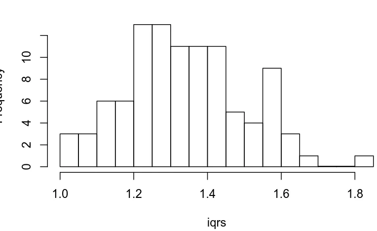
8.5.1 Plot of simulated IQRs. . . 201

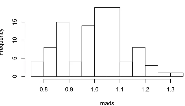
8.5.2 Plot of simulated MADs . . . 202

9.1.1 Capture-recapture experiment . . . 207

9.1.2 Assorted likelihood functions for fishing, part two . . . 209

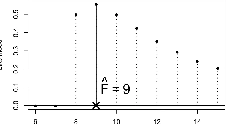
9.1.3 Species maximum likelihood . . . 210

9.2.1 Simulated confidence intervals . . . 216

9.2.2 Confidence interval plot for thePlantGrowthdata. . . 219

(14)

10.3.1 Hypothesis test plot based onnormal.and.t.distfrom theHHpackage . . . 238

10.6.1 Between group versus within group variation . . . 244

10.6.2 Between group versus within group variation . . . 245

10.6.3 SomeFplots from theHHpackage . . . 246

10.7.1 Plot of significance level and power . . . 247

11.1.1 Philosophical foundations of SLR . . . 251

11.1.2 Scatterplot ofdistversusspeedfor thecarsdata . . . 252

11.2.1 Scatterplot with added regression line for thecarsdata . . . 255

11.2.2 Scatterplot with confidence/prediction bands for thecarsdata . . . 263

11.4.1 Normal q-q plot of the residuals for thecarsdata . . . 269

11.4.2 Plot of standardized residuals against the fitted values for thecarsdata. . . . 271

11.4.3 Plot of the residuals versus the fitted values for thecarsdata . . . 273

11.5.1 Cook’s distances for thecarsdata . . . 280

11.5.2 Diagnostic plots for thecarsdata. . . 281

12.1.1 Scatterplot matrix oftreesdata . . . 287

12.1.2 3D scatterplot with regression plane for thetreesdata . . . 289

12.4.1 Scatterplot ofVolumeversusGirthfor thetreesdata . . . 300

12.4.2 A quadratic model for thetreesdata . . . 303

12.6.1 A dummy variable model for thetreesdata . . . 309

13.2.1 Bootstrapping the standard error of the mean, simulated data . . . 322

(15)

List of Tables

4.1 Samplingkfromnobjects withurnsamples . . . 89

4.2 Rolling two dice. . . 94

5.1 Correspondence betweenstatsanddistr . . . 121

7.1 MaximumUand sumVof a pair of dice rolls (X,Y) . . . 168

7.2 Joint values ofU=max(X,Y) andV=X+Y . . . 168

7.3 The joint PMF of (U,V) . . . 168

E.1 Set operations . . . 361

E.2 Differentiation rules. . . 363

E.3 Some derivatives . . . 363

E.4 Some integrals (constants of integration omitted) . . . 364

(16)

(17)

An Introduction to Probability and

Statistics

This chapter has proved to be the hardest to write, by far. The trouble is that there is so much to say – and so many people have already said it so much better than I could. When I get something I like I will release it here.

In the meantime, there is a lot of information already available to a person with an Internet connection. I recommend to start at Wikipedia, which is not a flawless resource but it has the main ideas with links to reputable sources.

In my lectures I usually tell stories about Fisher, Galton, Gauss, Laplace, Quetelet, and the Chevalier de Mere.

1.1

Probability

The common folklore is that probability has been around for millennia but did not gain the attention of mathematicians until approximately 1654 when the Chevalier de Mere had a question regarding the fair division of a game’s payoffto the two players, if the game had to end prematurely.

1.2

Statistics

Statistics concerns data; their collection, analysis, and interpretation. In this book we distinguish between two types of statistics: descriptive and inferential.

Descriptive statistics concerns the summarization of data. We have a data set and we would like to describe the data set in multiple ways. Usually this entails calculating numbers from the data, called descriptive measures, such as percentages, sums, averages, and so forth.

Inferential statistics does more. There is an inference associated with the data set, a conclusion drawn about the population from which the data originated.

I would like to mention that there are two schools of thought of statistics: frequentist and bayesian. The difference between the schools is related to how the two groups interpret the under-lying probability (see Section4.3). The frequentist school gained a lot of ground among statisti-cians due in large part to the work of Fisher, Neyman, and Pearson in the early twentieth century.

(18)

That dominance lasted until inexpensive computing power became widely available; nowadays the bayesian school is garnering more attention and at an increasing rate.

This book is devoted mostly to the frequentist viewpoint because that is how I was trained, with the conspicuous exception of Sections4.8and7.3. I plan to add more bayesian material in later editions of this book.

(19)

An Introduction to

R

2.1

Downloading and Installing

R

The instructions for obtainingRlargely depend on the user’s hardware and operating system. TheR

Project has written anRInstallation and Administration manual with complete, precise instructions about what to do, together with all sorts of additional information. The following is just a primer to get a person started.

2.1.1

Installing

R

Visit one of the links below to download the latest version ofRfor your operating system: Microsoft Windows: http://cran.r-project.org/bin/windows/base/

MacOS: http://cran.r-project.org/bin/macosx/

Linux: http://cran.r-project.org/bin/linux/

On Microsoft Windows, click the R-x.y.z.exeinstaller to start installation. When it asks for "Customized startup options", specifyYes. In the next window, be sure to select the SDI (single document interface) option; this is useful later when we discuss three dimensional plots with the rglpackage [1].

InstallingRon a USB drive (Windows) With this option you can useRportably and without administrative privileges. There is an entry in theR for Windows FAQ about this. Here is the procedure I use:

1. Download the Windows installer above and start installation as usual. When it askswhereto install, navigate to the top-level directory of the USB drive instead of the defaultCdrive. 2. When it asks whether to modify the Windows registry, uncheck the box; we do NOT want to

tamper with the registry.

3. After installation, change the name of the folder fromR-x.y.zto just plainR. (Even quicker: do this in step 1.)

(20)

4. Download the following shortcut to the top-level directory of the USB drive, right beside the Rfolder, not inside the folder.

http://ipsur.r-forge.r-project.org/book/download/R.exe

Use the downloaded shortcut to runR.

Steps 3 and 4 are not required but save you the trouble of navigating to theR-x.y.z/bindirectory to double-clickRgui.exeevery time you want to run the program. It is useless to create your own shortcut toRgui.exe. Windows does not allow shortcuts to have relative paths; they always have a drive letter associated with them. So if you make your own shortcut and plug your USB drive into someothermachine that happens to assign your drive a different letter, then your shortcut will no longer be pointing to the right place.

2.1.2

Installing and Loading Add-on Packages

There are base packages (which come withR automatically), and contributedpackages (which must be downloaded for installation). For example, on the version ofRbeing used for this docu-ment the default base packages loaded at startup are

> getOption("defaultPackages")

[1] "datasets" "utils" "grDevices" "graphics" "stats" "methods"

The base packages are maintained by a select group of volunteers, called “RCore”. In addi-tion to the base packages, there are literally thousands of addiaddi-tional contributed packages written by individuals all over the world. These are stored worldwide on mirrors of the Comprehensive

RArchive Network, orCRAN for short. Given an active Internet connection, anybody is free to download and install these packages and even inspect the source code.

To install a package named foo, open upRand typeinstall.packages("foo"). To in-stallfooand additionally install all of the other packages on which foodepends, instead type install.packages("foo", depends = TRUE).

The general commandinstall.packages()will (on most operating systems) open a window containing a huge list of available packages; simply choose one or more to install.

No matter how many packages are installed onto the system, each one must first be loaded for use with thelibraryfunction. For instance, theforeignpackage [18] contains all sorts of functions needed to import data sets intoRfrom other software such as SPSS, SAS,etc.. But none of those functions will be available until the commandlibrary(foreign)is issued.

Typelibrary()at the command prompt (described below) to see a list of all available pack-ages in your library.

For complete, precise information regarding installation of Rand add-on packages, see theR

Installation and Administration manual,http://cran.r-project.org/manuals.html.

2.2

Communicating with

R

(21)

RGui_(Microsoftr_Windows)

Terminal

Emacs/ESS, XEmacs JGR

Multiple lines at a time For longer programs (calledscripts) there is too much code to write all at once at the command prompt. Furthermore, for longer scripts it is convenient to be able to only modify a certain piece of the script and run it again inR. Programs calledscript editors are specially designed to aid the communication and code writing process. They have all sorts of helpful features includingRsyntax highlighting, automatic code completion, delimiter matching, and dynamic help on theRfunctions as they are being written. Even more, they often have all of the text editing features of programs like MicrosoftrWord. Lastly, most script editors are fully customizable in the sense that the user can customize the appearance of the interface to choose what colors to display, when to display them, and how to display them.

R_{Editor (Windows):} _{In Microsoftr}_Windows,_R_{Gui has its own built-in script editor, called}_R

Editor. From the console window, selectFile⊲New Script.A script window opens, and the lines of code can be written in the window. When satisfied with the code, the user highlights all of the commands and pressesCtrl+R. The commands are automatically run at once inR

and the output is shown. To save the script for later, clickFile⊲Save as...inREditor. The script can be reopened later withFile⊲Open Script...inRGui. Note thatREditor does not have the fancy syntax highlighting that the others do.

RWinEdt: This option is coordinated with WinEdt for LA_{TEX and has additional features such as} code highlighting, remote sourcing, and a ton of other things. However, one first needs to download and install a shareware version of another program, WinEdt, which is only free for a while – pop-up windows will eventually appear that ask for a registration code. RWinEdt is nevertheless a very fine choice if you already own WinEdt or are planning to purchase it in the near future.

Tinn-R/Sciviews-K: This one is completely free and has all of the above mentioned options and more. It is simple enough to use that the user can virtually begin working with it immediately after installation. But Tinn-Rproper is only available for MicrosoftrWindows operating systems. If you are on MacOS or Linux, a comparable alternative is Sci-Views - Komodo Edit.

Emacs/ESS: Emacs is an all purpose text editor. It can do absolutely anything with respect to modifying, searching, editing, and manipulating, text. And if Emacs can’t do it, then you can write a program that extends Emacs to do it. Once such extension is calledESS, which stands forEmacsSpeaksStatistics. With ESS a person can speak toR,do all of the tricks that the other script editors offer, and much, much, more. Please see the following for installation details, documentation, reference cards, and a whole lot more:

(22)

Fair warning: if you want to try Emacs and if you grew up with MicrosoftrWindows or Macintosh, then you are going to need to relearn everything you thought you knew about computers your whole life. (Or, since Emacs is completely customizable, you can reconfigure Emacs to behave the way you want.) I have personally experienced this transformation and I will never go back. JGR (read “Jaguar”): This one has the bells and whistles of RGuiplus it is based on Java, so

it works on multiple operating systems. It has its own script editor likeREditor but with additional features such as syntax highlighting and code-completion. If you do not use MicrosoftrWindows (or even if you do) you definitely want to check out this one.

Kate, Bluefish,etc. There are literally dozens of other text editors available, many of them free, and each has its own (dis)advantages. I only have mentioned the ones with which I have had substantial personal experience and have enjoyed at some point. Play around, and let me know what you find.

Graphical User Interfaces (GUIs) By the word “GUI” I mean an interface in which the user communicates withRby way of points-and-clicks in a menu of some sort. Again, there are many, many options and I only mention ones that I have used and enjoyed. Some of the other more popular script editors can be downloaded from theR-Project website athttp://www.sciviews. org/_rgui/. On the left side of the screen (underProjects) there are several choices available.

RCommander provides a point-and-click interface to many basic statistical tasks. It is called the “Commander” because every time one makes a selection from the menus, the code corre-sponding to the task is listed in the output window. One can take this code, copy-and-paste it to a text file, then re-run it again at a later time without theRCommander’s assistance. It is well suited for the introductory level. Rcmdralso allows for user-contributed “Plugins” which are separate packages onCRANthat add extra functionality to theRcmdrpackage. The plugins are typically named with the prefixRcmdrPluginto make them easy to identify in theCRANpackage list. One such plugin is the

RcmdrPlugin.IPSURpackage which accompanies this text.

Poor Man’s GUI is an alternative to theRcmdrwhich is based on GTk instead of Tcl/Tk. It has been a while since I used it but I remember liking it very much when I did. One thing that stood out was that the user could drag-and-drop data sets for plots. See here for more information:http://wiener.math.csi.cuny.edu/pmg/.

Rattle is a data mining toolkit which was designed to manage/analyze very large data sets, but it provides enough other general functionality to merit mention here. See [91] for more information.

Deducer is relatively new and shows promise from what I have seen, but I have not actually used it in the classroom yet.

2.3

Basic

R

Operations and Concepts

(23)

all new users ofRread that document, but bear in mind that there are concepts mentioned which will be unfamiliar to the beginner.

Below are some of the most basic operations that can be done withR. Almost every book about

Rbegins with a section like the one below; look around to see all sorts of things that can be done at this most basic level.

2.3.1

Arithmetic

> 2 + 3 # add

[1] 5

> 4 * 5 / 6 # multiply and divide

[1] 3.333333

> 7^8 # 7 to the 8th power

[1] 5764801

Notice the comment character#. Anything typed after a#symbol is ignored byR. We know that 20/6 is a repeating decimal, but the above example shows only 7 digits. We can change the number of digits displayed withoptions:

> options(digits = 16)

> 10/3 # see more digits

[1] 3.333333333333333

> sqrt(2) # square root

[1] 1.414213562373095

> exp(1) # Euler's constant, e

[1] 2.718281828459045

> pi

[1] 3.141592653589793

> options(digits = 7) # back to default

Note that it is possible to setdigitsup to 22, but setting them over 16 is not recommended (the extra significant digits are not necessarily reliable). Above notice thesqrtfunction for square roots and theexpfunction for powers of e, Euler’s number.

2.3.2

Assignment, Object names, and Data types

(24)

> x <- 7*41/pi # don't see the calculated value > x # take a look

[1] 91.35494

When choosing a variable name you can use letters, numbers, dots “.”, or underscore “_” characters. You cannot use mathematical operators, and a leading dot may not be followed by a number. Examples of valid names are: x,x1,y.value, andy_hat. (More precisely, the set of allowable characters in object names depends on one’s particular system and locale; see An Introduction toRfor more discussion on this.)

Objects can be of manytypes,modes, andclasses. At this level, it is not necessary to investigate all of the intricacies of the respective types, but there are some with which you need to become familiar:

integer: the values 0,_±1,_±2, . . . ; these are represented exactly byR.

double: real numbers (rational and irrational); these numbers are not represented exactly (save integers or fractions with a denominator that is a power of 2, see [85]).

character: elements that are wrapped with pairs of"or';

logical: includesTRUE,FALSE, andNA(which are reserved words); theNAstands for “not avail-able”,i.e., a missing value.

You can determine an object’s type with thetypeoffunction. In addition to the above, there is the complexdata type:

> sqrt(-1) # isn't defined

[1] NaN

> sqrt(-1+0i) # is defined

[1] 0+1i

> sqrt(as.complex(-1)) # same thing

[1] 0+1i

> (0 + 1i)^2 # should be -1

[1] -1+0i

> typeof((0 + 1i)^2)

[1] "complex"

Note that you can just type(1i)^2to get the same answer. TheNaNstands for “not a number”; it is represented internally asdouble.

2.3.3

Vectors

(25)

Entering data vectors

1. c: If you would like to enter the data 74,31,95,61,76,34,23,54,96into R, you may create a data vector with thecfunction (which is short forconcatenate).

> x <- c(74, 31, 95, 61, 76, 34, 23, 54, 96) > x

[1] 74 31 95 61 76 34 23 54 96

The elements of a vector are usually coerced byRto the the most general type of any of the elements, so if you doc(1, "2")then the result will bec("1", "2").

2. scan: This method is useful when the data are stored somewhere else. For instance, you may typex <- scan()at the command prompt andRwill display1:to indicate that it is waiting for the first data value. Type a value and pressEnter, at which pointRwill display 2:, and so forth. Note that entering an empty line stops the scan. This method is especially handy when you have a column of values, say, stored in a text file or spreadsheet. You may copy and paste them all at the1:prompt, andRwill store all of the values instantly in the vectorx.

3. repeated data; regular patterns: theseqfunction will generate all sorts of sequences of num-bers. It has the argumentsfrom,to,by, andlength.outwhich can be set in concert with one another. We will do a couple of examples to show you how it works.

> seq(from = 1, to = 5)

[1] 1 2 3 4 5

> seq(from = 2, by = -0.1, length.out = 4)

[1] 2.0 1.9 1.8 1.7

Note that we can get the first line much quicker with the colon operator:

> 1:5

[1] 1 2 3 4 5

The vectorLETTERShas the 26 letters of the English alphabet in uppercase andlettershas all of them in lowercase.

Indexing data vectors Sometimes we do not want the whole vector, but just a piece of it. We can access the intermediate parts with the[]operator. Observe (withxdefined above)

> x[1]

[1] 74

(26)

[1] 31 95 61

> x[c(1, 3, 4, 8)]

[1] 74 95 61 54

> x[-c(1, 3, 4, 8)]

[1] 31 76 34 23 96

Notice that we used the minus sign to specify those elements that we donotwant.

> LETTERS[1:5]

[1] "A" "B" "C" "D" "E"

> letters[-(6:24)]

[1] "a" "b" "c" "d" "e" "y" "z"

2.3.4

Functions and Expressions

A function takes arguments as input and returns an object as output. There are functions to do all sorts of things. We show some examples below.

> x <- 1:5 > sum(x)

[1] 15

> length(x)

[1] 5

> min(x)

[1] 1

> mean(x) # sample mean

[1] 3

> sd(x) # sample standard deviation

[1] 1.581139

It will not be long before the user starts to wonder how a particular function is doing its job, and sinceRis open-source, anybody is free to look under the hood of a function to see how things are calculated. For detailed instructions see the article “Accessing the Sources” by Uwe Ligges [60]. In short:

1. Type the name of the function without any parentheses or arguments. If you are lucky then the code for the entire function will be printed, right there looking at you. For instance, suppose that we would like to see how theintersectfunction works:

(27)

function (x, y) {

y <- as.vector(y)

unique(y[match(as.vector(x), y, 0L)]) }

<environment: namespace:base>

2. If instead it showsUseMethod("something")then you will need to choose theclassof the object to be inputted and next look at themethodthat will bedispatchedto the object. For instance, typingrevsays

> rev

function (x) UseMethod("rev")

<environment: namespace:base>

The output is telling us that there are multiple methods associated with therevfunction. To see what these are, type

> methods(rev)

[1] rev.default rev.dendrogram*

Non-visible functions are asterisked

Now we learn that there are two differentrev(x)functions, only one of which being chosen at each call depending on whatxis. There is one fordendrogramobjects and adefault method for everything else. Simply type the name to see what each method does. For example, thedefaultmethod can be viewed with

> rev.default

function (x)

if (length(x)) x[length(x):1L] else x <environment: namespace:base>

3. Some functions are hidden by a namespace(see An Introduction to R [85]), and are not visible on the first try. For example, if we try to look at the code for wilcox.test(see Chapter15) we get the following:

> wilcox.test

function (x, ...)

(28)

> methods(wilcox.test)

[1] wilcox.test.default* wilcox.test.formula*

Non-visible functions are asterisked

If we were to trywilcox.test.defaultwe would get a “not found” error, because it is hidden behind the namespace for the packagestats(shown in the last line when we tried wilcox.test). In cases like these we prefix the package name to the front of the func-tion name with three colons; the commandstats:::wilcox.test.defaultwill show the source code, omitted here for brevity.

4. If it shows.Internal(something)or.Primitive("something"), then it will be necessary to download the source code of R(which is nota binary version with an.exeextension) and search inside the code there. See Ligges [60] for more discussion on this. An example isexp:

> exp

function (x) .Primitive("exp")

Be warned that most of the.Internalfunctions are written in other computer languages which the beginner may not understand, at least initially.

2.4

Getting Help

When you are usingR, it will not take long before you find yourself needing help. Fortunately,

Rhas extensive help resources and you should immediately become familiar with them. Begin by clickingHelponRgui. The following options are available.

• Console: gives useful shortcuts, for instance,Ctrl+L, to clear theRconsole screen. • FAQ onR_{: frequently asked questions concerning general}_R_operation.

• FAQ on R _{for Windows: frequently asked questions about} _R_{, tailored to the Microsoft}

Windows operating system.

• Manuals: technical manuals about all features of theRsystem including installation, the complete language definition, and add-on packages.

• Rfunctions (text). . .: use this if you know theexactname of the function you want to know more about, for example,meanorplot. Typingmeanin the window is equivalent to typing help("mean")at the command line, or more simply,?mean. Note that this method only works if the function of interest is contained in a package that is already loaded into the search path withlibrary.

(29)

• Search help. . .: use this if you do not know the exact name of the function of interest, or if the function is in a package that has not been loaded yet. For example, you may enterplo and a text window will return listing all the help files with an alias, concept, or title matching ‘plo’ using regular expression matching; it is equivalent to typinghelp.search("plo") at the command line. The advantage is that you do not need to know the exact name of the function; the disadvantage is that you cannot point-and-click the results. Therefore, one may wish to use the HTML Help search engine instead. An equivalent way is??ploat the command line.

• search.r-project.org. . .: this will search for words in help lists and email archives of theR

Project. It can be very useful for finding other questions that other users have asked.

• Apropos. . .: use this for more sophisticated partial name matching of functions. See?apropos for details.

On the help pages for a function there are sometimes “Examples” listed at the bottom of the page, which will work if copy-pasted at the command line (unless marked otherwise). The example function will run the code automatically, skipping the intermediate step. For instance, we may try example(mean)to see a few examples of how themeanfunction works.

2.4.1

R

Help Mailing Lists

There are several mailing lists associated withR, and there is a huge community of people that read and answer questions related toR. See herehttp://www.r-project.org/mail.htmlfor an idea of what is available. Particularly pay attention to the bottom of the page which lists several special interest groups (SIGs) related toR.

Bear in mind that Ris free software, which means that it was written by volunteers, and the people that frequent the mailing lists are also volunteers who are not paid by customer support fees. Consequently, if you want to use the mailing lists for free advice then you must adhere to some basic etiquette, or else you may not get a reply, or even worse, you may receive a reply which is a bit less cordial than you are used to. Below are a few considerations:

1. Read the FAQ (http://cran.r-project.org/faqs.html). Note that there are different FAQs for different operating systems. You should read these now, even without a question at the moment, to learn a lot about the idiosyncrasies ofR.

2. Search the archives. Even if your question is not a FAQ, there is a very high likelihood that your question has been asked before on the mailing list. If you want to know about topicfoo, then you can doRSiteSearch("foo")to search the mailing list archives (and the online help) for it.

3. Do a Google search and anRSeek.orgsearch.

If your question is not a FAQ, has not been asked onR-help before, and does not yield to a Google (or alternative) search, then, and only then, should you even consider writing toR-help. Below are a few additional considerations.

(30)

2. Get rid of the command prompts (>) from output. Readers of your message will take the text from your mail and copy-paste into anRsession. If you make the readers’ job easier then it will increase the likelihood of a response.

3. Questions are often related to a specific data set, and the best way to communicate the data is with adumpcommand. For instance, if your question involves data stored in a vectorx, you can typedump("x","")at the command prompt and copy-paste the output into the body of your email message. Then the reader may easily copy-paste the message from your email intoRandxwill be available to him/her.

4. Sometimes the answer the question is related to the operating system used, the attached packages, or the exact version of R being used. ThesessionInfo() command collects all of this information to be copy-pasted into an email (and the Posting Guide requests this information). See AppendixAfor an example.

2.5

External Resources

There is a mountain of information on the Internet aboutR. Below are a few of the important ones. TheRProject for Statistical Computing: (http://www.r-project.org/) Go here first. The ComprehensiveR_{Archive Network:} _{(http://cran.r-project.org/) This is where}_R

is stored along with thousands of contributed packages. There are also loads of contributed information (books, tutorials,etc.). There are mirrors all over the world with duplicate infor-mation.

R-Forge: (http://r-forge.r-project.org/) This is another location whereRpackages are stored. Here you can find development code which has not yet been released toCRAN.

RWiki: (http://wiki.r-project.org/rwiki/doku.php) There are many tips and tricks listed here. If you find a trick of your own, login and share it with the world.

Other: theRGraph Gallery (http://addictedtor.free.fr/graphiques/) andRGraphical Manual (http://bm2.genes.nig.ac.jp/RGM2/index.php) have literally thousands of graphs to peruse. RSeek (http://www.rseek.org) is a search engine based on Google specifically tailored forRqueries.

2.6

Other Tips

It is unnecessary to retype commands repeatedly, sinceRremembers what you have recently en-tered on the command line. On the MicrosoftrWindows RGui, to cycle through the previous commands just push the_↑(up arrow) key. On Emacs/ESS the command isM-p(which means hold down theAltbutton and press “p”). More generally, the commandhistory()will show a whole list of recently entered commands.

(31)

• Another use ofscan is when you have a long list of numbers (separated by spaces or on different lines) already typed somewhere else, say in a text file. To enter all the data in one fell swoop, first highlight and copy the list of numbers to the Clipboard withEdit ⊲Copy

(or by right-clicking and selecting Copy). Next type thex <- scan()command in theR

console, and paste the numbers at the1:prompt withEdit⊲Paste. All of the numbers will automatically be entered into the vectorx.

• The commandCtrl+lclears the screen in the MicrosoftrWindowsRGui. The comparable command for Emacs/ESS is

• Once you useRfor awhile there may be some commands that you wish to run automatically wheneverRstarts. These commands may be saved in a file calledRprofile.sitewhich is usually in the etcfolder, which lives in the R home directory (which on Microsoftr Windows usually isC:\Program Files\R). Alternatively, you can make a file.Rprofile to be stored in the user’s home directory, or anywhereRis invoked. This allows for multiple configurations for different projects or users. See “Customizing the Environment” of An Introduction toRfor more details.

• When exiting R the user is given the option to “save the workspace”. I recommend that beginners DO NOT save the workspace when quitting. If Yes is selected, then all of the objects and data currently inR’s memory is saved in a file located in the working directory called.RData. This file is then automatically loaded the next timeRstarts (in which case

(32)

(33)

Data Description

In this chapter we introduce the different types of data that a statistician is likely to encounter, and in each subsection we give some examples of how to display the data of that particular type. Once we see how to display data distributions, we next introduce the basic properties of data distributions. We qualitatively explore several data sets. Once that we have intuitive properties of data sets, we next discuss how we may numerically measure and describe those properties with descriptive statistics.

What do I want them to know?

• different data types, such as quantitative versus qualitative, nominal versus ordinal, and dis-crete versus continuous

• basic graphical displays for assorted data types, and some of their (dis)advantages

• fundamental properties of data distributions, including center, spread, shape, and crazy ob-servations

• methods to describe data (visually/numerically) with respect to the properties, and how the methods differ depending on the data type

• all of the above in the context of grouped data, and in particular, the concept of a factor

3.1

Types of Data

Loosely speaking, a datum is any piece of collected information, and a data set is a collection of data related to each other in some way. We will categorize data into five types and describe each in turn:

Quantitative data associated with a measurement of some quantity on an observational unit, Qualitative data associated with some quality or property of the observational unit,

(34)

Missing data that should be there but are not, and Other types everything else under the sun.

In each subsection we look at some examples of the type in question and introduce methods to display them.

3.1.1

Quantitative data

Quantitative data are any data that measure or are associated with a measurement of the quantity of something. They invariably assume numerical values. Quantitative data can be further subdivided into two categories.

• Discrete datatake values in a finite or countably infinite set of numbers, that is, all possible values could (at least in principle) be written down in an ordered list. Examples include: counts, number of arrivals, or number of successes. They are often represented by integers, say, 0, 1, 2,etc..

• Continuous datatake values in an interval of numbers. These are also known as scale data, interval data, or measurement data. Examples include: height, weight, length, time, etc. Continuous data are often characterized by fractions or decimals: 3.82, 7.0001, 45₈,etc.. Note that the distinction between discrete and continuous data is not always clear-cut. Sometimes it is convenient to treat data as if they were continuous, even though strictly speaking they are not continuous. See the examples.

Example 3.1. Annual Precipitation in US Cities. The vectorprecipcontains average amount of rainfall (in inches) for each of 70 cities in the United States and Puerto Rico. Let us take a look at the data:

> str(precip)

Named num [1:70] 67 54.7 7 48.5 14 17.2 20.7 13 43.4 40.2 ...

- attr(*, "names")= chr [1:70] "Mobile" "Juneau" "Phoenix" "Little Rock" ...

> precip[1:4]

Mobile Juneau Phoenix Little Rock

67.0 54.7 7.0 48.5

The output shows thatprecipis a numeric vector which has beennamed, that is, each value has a name associated with it (which can be set with thenamesfunction). These are quantitative continuous data.

Example 3.2. Lengths of Major North American Rivers.The U.S. Geological Survey recorded the lengths (in miles) of several rivers in North America. They are stored in the vectorriversin thedatasetspackage (which ships with baseR). See?rivers. Let us take a look at the data with thestrfunction.

> str(rivers)

(35)

The output says thatriversis a numeric vector of length 141, and the first few values are 735, 320, 325,etc. These data are definitely quantitative and it appears that the measurements have been rounded to the nearest mile. Thus, strictly speaking, these are discrete data. But we will find it convenient later to take data like these to be continuous for some of our statistical procedures. Example 3.3. Yearly Numbers of Important Discoveries. The vectordiscoveries contains numbers of “great” inventions/discoveries in each year from 1860 to 1959, as reported by the 1975 World Almanac. Let us take a look at the data:

> str(discoveries)

Time-Series [1:100] from 1860 to 1959: 5 3 0 2 0 3 2 3 6 1 ...

> discoveries[1:4]

[1] 5 3 0 2

The output is telling us thatdiscoveriesis atime series(see Section3.1.5for more) of length 100. The entries are integers, and since they represent counts this is a good example of discrete quantitative data. We will take a closer look in the following sections.

Displaying Quantitative Data

One of the first things to do when confronted by quantitative data (or any data, for that matter) is to make some sort of visual display to gain some insight into the data’s structure. There are almost as many display types from which to choose as there are data sets to plot. We describe some of the more popular alternatives.

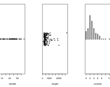
Strip charts (also known as Dot plots) These can be used for discrete or continuous data, and usually look best when the data set is not too large. Along the horizontal axis is a numerical scale above which the data values are plotted. We can do it inRwith a call to thestripchartfunction. There are three available methods.

overplot plots ties covering each other. This method is good to display only the distinct values assumed by the data set.

jitter adds some noise to the data in theydirection in which case the data values are not covered up by ties.

stack plots repeated values stacked on top of one another. This method is best used for discrete data with a lot of ties; if there are no repeats then this method is identical to overplot. See Figure3.1.1, which is produced by the following code.

> stripchart(precip, xlab = "rainfall")

(36)

10 30 50

rainfall

0 1000 2500

length

0 2 4 6 8 12

number

Figure 3.1.1: Strip charts of theprecip,rivers, anddiscoveriesdata

The first graph uses theoverplotmethod, the second thejittermethod, and the third thestackmethod.

The leftmost graph is a strip chart of theprecipdata. The graph shows tightly clustered values in the middle with some others falling balanced on either side, with perhaps slightly more falling to the left. Later we will call this a symmetric distribution, see Section3.2.3. The middle graph is of theriversdata, a vector of length 141. There are several repeated values in the rivers data, and if we were to use the overplot method we would lose some of them in the display. This plot shows a what we will later call a right-skewed shape with perhaps some extreme values on the far right of the display. The third graph strip chartsdiscoveriesdata which are literally a textbook example of a right skewed distribution.

TheDOTplotfunction in theUsingRpackage [86] is another alternative.

(37)

of observations that fell into the bin.

These are one of the most common summary displays, and they are often misidentified as “Bar Graphs” (see below.) The scale on theyaxis can be frequency, percentage, or density (relative frequency). The term histogram was coined by Karl Pearson in 1891, see [66].

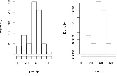
Example 3.4. Annual Precipitation in US Cities.We are going to take another look at theprecip data that we investigated earlier. The strip chart in Figure 3.1.1 suggested a loosely balanced distribution; let us now look to see what a histogram says.

There are many ways to plot histograms inR, and one of the easiest is with thehistfunction. The following code produces the plots in Figure3.1.2.

> hist(precip, main = "")

> hist(precip, freq = FALSE, main = "")

Notice the argument main = "", which suppresses the main title from being displayed – it would have said “Histogram ofprecip” otherwise. The plot on the left is a frequency histogram (the default), and the plot on the right is a relative frequency histogram (freq = FALSE).

Please be careful regarding the biggest weakness of histograms: the graph obtained strongly depends on the bins chosen. Choose another set of bins, and you will get a different histogram. Moreover, there are not any definitive criteria by which bins should be defined; the best choice for a given data set is the one which illuminates the data set’s underlying structure (if any). Luckily for us there are algorithms to automatically choose bins that are likely to display well, and more often than not the default bins do a good job. This is not always the case, however, and a responsible statistician will investigate many bin choices to test the stability of the display.

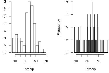
Example 3.5. Recall that the strip chart in Figure3.1.1suggested a relatively balanced shape to the precipdata distribution. Watch what happens when we change the bins slightly (with thebreaks argument tohist). See Figure3.1.3which was produced by the following code.

> hist(precip, breaks = 10, main = "") > hist(precip, breaks = 200, main = "")

The leftmost graph (withbreaks = 10) shows that the distribution is not balanced at all. There are two humps: a big one in the middle and a smaller one to the left. Graphs like this often indicate some underlying group structure to the data; we could now investigate whether the cities for which rainfall was measured were similar in some way, with respect to geographic region, for example.

The rightmost graph in Figure3.1.3shows what happens when the number of bins is too large: the histogram is too grainy and hides the rounded appearance of the earlier histograms. If we were to continue increasing the number of bins we would eventually get all observed bins to have exactly one element, which is nothing more than a glorified strip chart.

(38)

precip

Frequency

0

20

40

60

0

5

10

15

20

25

precip

Density

0

20

40

60

0.000

0.010

0.020

0.030

(39)

precip

Frequency

10

30

50

70

0

2

4

6

8

10

12

14

precip

Frequency

10

30

50

0

1

2

3

4

(40)

Example 3.6. UKDriverDeathsis a time series that contains the total car drivers killed or se-riously injured in Great Britain monthly from Jan 1969 to Dec 1984. See?UKDriverDeaths. Compulsory seat belt use was introduced on January 31, 1983. We construct a stem and leaf dia-gram inRwith thestem.leaffunction from theaplpackpackage [92].

> library(aplpack)

> stem.leaf(UKDriverDeaths, depth = FALSE)

1 | 2: represents 120 leaf unit: 10

n: 192 10 | 57

11 | 136678 12 | 123889

13 | 0255666888899

14 | 00001222344444555556667788889 15 | 0000111112222223444455555566677779 16 | 01222333444445555555678888889 17 | 11233344566667799

18 | 00011235568 19 | 01234455667799 20 | 0000113557788899 21 | 145599

22 | 013467 23 | 9 24 | 7 HI: 2654

The display shows a more or less balanced mound-shaped distribution, with one or maybe two humps, a big one and a smaller one just to its right. Note that the data have been rounded to the tens place so that each datum gets only one leaf to the right of the dividing line.

Notice that thedepths have been suppressed. To learn more about this option and many others, see Section3.4. Unlike a histogram, the original data values may be recovered from the stemplot display – modulo the rounding – that is, starting from the top and working down we can read off

the data values 1050, 1070, 1110, 1130,etc.

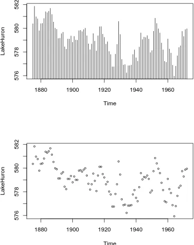
Index plot Done with theplot function. These are good for plotting data which are ordered, for example, when the data are measured over time. That is, the first observation was measured at time 1, the second at time 2,etc. It is a two dimensional plot, in which the index (or time) is the xvariable and the measured value is theyvariable. There are several plotting methods for index plots, and we discuss two of them:

spikes: draws a vertical line from thex-axis to the observation height (type = "h"). points: plots a simple point at the observation height (type = "p").

(41)

> plot(LakeHuron, type = "h") > plot(LakeHuron, type = "p")

The plots show an overall decreasing trend to the observations, and there appears to be some seasonal variation that increases over time.

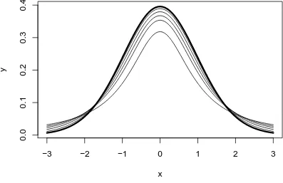
Density estimates

3.1.2

Qualitative Data, Categorical Data, and Factors

Qualitative data are simply any type of data that are not numerical, or do not represent numerical quantities. Examples of qualitative variables include a subject’s name, gender, race/ethnicity, po-litical party, socioeconomic status, class rank, driver’s license number, and social security number (SSN).

Please bear in mind that some data lookto be quantitative but are not, because they do not represent numerical quantities and do not obey mathematical rules. For example, a person’s shoe size is typically written with numbers: 8, or 9, or 12, or 121

2. Shoe size is not quantitative, however, because if we take a size 8 and combine with a size 9 we do not get a size 17.

Some qualitative data serve merely toidentifythe observation (such a subject’s name, driver’s license number, or SSN). This type of data does not usually play much of a role in statistics. But other qualitative variables serve tosubdividethe data set into categories; we call thesefactors. In the above examples, gender, race, political party, and socioeconomic status would be considered factors (shoe size would be another one). The possible values of a factor are called itslevels. For instance, the factorgenderwould have two levels, namely, male and female. Socioeconomic status typically has three levels: high, middle, and low.

Factors may be of two types:nominalandordinal. Nominal factors have levels that correspond to names of the categories, with no implied ordering. Examples of nominal factors would be hair color, gender, race, or political party. There is no natural ordering to “Democrat” and “Republican”; the categories are just names associated with different groups of people.

In contrast, ordinal factors have some sort of ordered structure to the underlying factor levels. For instance, socioeconomic status would be an ordinal categorical variable because the levels cor-respond to ranks associated with income, education, and occupation. Another example of ordinal categorical data would be class rank.

Factors have special status inR. They are represented internally by numbers, but even when they are written numerically their values do not convey any numeric meaning or obey any mathematical rules (that is, Stage III cancer is not Stage I cancer+Stage II cancer).

Example 3.8. Thestate.abbvector gives the two letter postal abbreviations for all 50 states.

> str(state.abb)

chr [1:50] "AL" "AK" "AZ" "AR" "CA" "CO" "CT" "DE" ...

These would be ID data. Thestate.namevector lists all of the complete names and those data would also be ID.

(42)

Time

Lak

eHuron

1880

1900

1920

1940

1960

576

578

580

582

● ● ● ● ● ●● ● ●●●●_● ● ●● ●● ●● ● ● ●●● ● ● ●● ●●●●● ● ● ● ● ● ● ● ● ●● ● ● ●● ● ● ●● ● ● ● ● ● ●● ● ●●● ● ● ● ● ● ● ●●●●● ●● ● ● ● ● ● ● ● ●● ● ● ● ● ● ● ● ●● ● ● ●●

Time

Lak

eHuron

1880

1900

1920

1940

1960

576

578

580

582

(43)

state.regiondata lists each of the 50 states and the region to which it belongs, be it Northeast, South, North Central, or West. See?state.region.

> str(state.region)

Factor w/ 4 levels "Northeast","South",..: 2 4 4 2 4 4 1 2 2 2 ...

> state.region[1:5]

[1] South West West South West

Levels: Northeast South North Central West

Thestroutput shows thatstate.regionis already stored internally as a factor and it lists a couple of the factor levels. To see all of the levels we printed the first five entries of the vector in the second line.need to print a piece of the from

Displaying Qualitative Data

Tables One of the best ways to summarize qualitative data is with a table of the data values. We may count frequencies with thetablefunction or list proportions with theprop.tablefunction (whose input is a frequency table). In theRCommander you can do it withStatistics⊲Frequency Distribution. . . .Alternatively, to look at tables for all factors in theActive data setyou can do

Statistics⊲Summaries⊲Active Dataset.

> Tbl <- table(state.division) > Tbl # frequencies

state.division

New England Middle Atlantic South Atlantic

6 3 8

East South Central West South Central East North Central

4 4 5

West North Central Mountain Pacific

7 8 5

> Tbl/sum(Tbl) # relative frequencies

state.division

0.12 0.06 0.16

0.08 0.08 0.10

0.14 0.16 0.10

> prop.table(Tbl) # same thing

state.division

0.12 0.06 0.16

0.08 0.08 0.10

(44)

Bar Graphs A bar graph is the analogue of a histogram for categorical data. A bar is displayed for each level of a factor, with the heights of the bars proportional to the frequencies of observations falling in the respective categories. A disadvantage of bar graphs is that the levels are ordered alphabetically (by default), which may sometimes obscure patterns in the display.

Example 3.10. U.S. State Facts and Features. The state.region data lists each of the 50 states and the region to which it belongs, be it Northeast, South, North Central, or West. See ?state.region. It is already stored internally as a factor. We make a bar graph with thebarplot function:

> barplot(table(state.region), cex.names = 0.5)

> barplot(prop.table(table(state.region)), cex.names = 0.5)

See Figure3.1.5. The display on the left is a frequency bar graph because theyaxis shows counts, while the display on the left is a relative frequency bar graph. The only difference between the two is the scale. Looking at the graph we see that the majority of the fifty states are in the South, followed by West, North Central, and finally Northeast. Over 30% of the states are in the South.

Notice thecex.namesargument that we used, above. It shrinks the names on thexaxis by 50% which makes them easier to read. See?parfor a detailed list of additional plot parameters.

Pareto Diagrams A pareto diagram is a lot like a bar graph except the bars are rearranged such that they decrease in height going from left to right. The rearrangement is handy because it can visually reveal structure (if any) in how fast the bars decrease – this is much more difficult when the bars are jumbled.

Example 3.11. U.S. State Facts and Features. Thestate.division data record the division (New England, Middle Atlantic, South Atlantic, East South Central, West South Central, East North Central, West North Central, Mountain, and Pacific) of the fifty states. We can make a pareto diagram with either theRcmdrPlugin.IPSURpackage or with thepareto.chartfunction from theqccpackage [77]. See Figure3.1.6. The code follows.

> library(qcc)

> pareto.chart(table(state.division), ylab = "Frequency")

Dot Charts These are a lot like a bar graph that has been turned on its side with the bars replaced by dots on horizontal lines. They do not convey any more (or less) information than the associated bar graph, but the strength lies in the economy of the display. Dot charts are so compact that it is easy to graph very complicated multi-variable interactions together in one graph. See Section

3.6. We will give an example here using the same data as above for comparison. The graph was produced by the following code.

> x <- table(state.region)

> dotchart(as.vector(x), labels = names(x))

(45)

Gambar

Figure 3.1.1: Strip charts of the precip, rivers, and discoveries data

Figure 3.1.2: (Relative) frequency histograms of the precip data

Figure 3.1.3: More histograms of the precip data

Figure 3.1.4: Index plots of the LakeHuron data

+7

Referensi

Unduh sekarang ( PDF - 412 Halaman - 1.32 MB )

Garis besar

Introduction to Probability and Statisti (3)

Dokumen terkait

PENTADBIRAN IPTS ISLAM CABARAN DAN HARAP

STRATEGI KOLEJ UNIVERSITI INSANIAH PEMBANGUNA N FIZIKAL PEMBANGUNA N FIZIKAL • Pembinaan kampus tetap oleh Kerajaan Negeri • Penswastaan pengurusan asrama • Perkongsian

Peranan dan Cabaran Masa Kini

Remaja adalah individu yang mempunyai peranan yang amat penting dalam membangunkan ekonomi negara.Merekalah yang akan menjadi pencetus pada generasi yang akan datang.Oleh sebab

this file 1962 7892 1 PB

Bаgi pеnеlitiаn sеlаnjutnyа dihаrаpkаn dаpаt mеnеliti dеngаn vаriаbеl - vаriаbеl lаin diluаr vаriаbеl yаng tеlаh ditеliti dаlаm pеnеlitiаn ini untuk mеmpеrolеh

Undangan Kualifikasi pangkalan lesung

Tempat : Kantor Dinas Pertambangan dan Energi Kabupaten Pelalawan Adapun daftar peserta yang dinyatakan Lulus mengikuti pembuktian kualifikasi sebagai berikut :.. No Nama

BA. Penjelasan Pekerjaan BAJO

Demikian Berita Acara ini dibuat dengan sebenar-benarnya untuk dipergunakan seperlunya. PANITIA

Munasabah dalam tafsir Mafatih al-Ghaib

Pada pembukaan surat diuraikan sifat-sifat orang mukmin yanr, percaya p1da al-Kitab yang tidak mengandung sedikitpun keragllan di dalamnya, maka di akhir surat ditutup dengan

Undangan Pembuktian Kualifikasi Pengadaan Pisang di Kab. Ngada

UNIT LAYANAN PENGADAAN (ULP) PROVINSI NUSA TENGGARA TIMUR Sekretariat : Biro Administrasi Pembangunan Setda Provinsi NTT.. (Kantor Gubernur Pertama

Pengaruh non performing financing dan dana pihak ketia terhadap return on assets : (studi kasus pada PT.Bank Rakyat Indonesia Syariah Periode 2008-2012)

[r]

Introduction to Probability and Statisti (3)