Volume 24, Number 2, 2009, 221– 231
THE IMPORTANCE OF PRECAUTIONARY SAVING MOTIVE
AMONG INDONESIAN HOUSEHOLDS
Ahmad Zafarullah Abdul Jalil
Universiti Utara Malaysia (zafar@uum.edu.my)
ABSTRACT
In the developing world, the population is frequently faced with numerous natural, economic, institutional and market risks. Because of these uncertainties, many individuals and households experience difficult periods of unexpected reduction in income. Using panel data from the Indonesian Family Life Survey (IFLS), this paper tests the existence of precautionary saving associated with income risk in Indonesia. The results of the estimation show that the uncertainty variable is not significantly related to the growth of consumption which signifies that Indonesian households do not constitute precautionary saving to smooth their consumption. The finding may be explained by the fact that Indonesian households have in their possession other type of support mechanisms based particularly on inter-generational and -communal solidarity.
Keywords: uncertainty, income risks, precautionary savings, consumption smoothing.
INTRODUCTION
In the developing world, the population is frequently faced with numerous natural, economic, institutional and market risks. Because of these uncertainties, many indivi-duals and households experience difficult periods of unexpected reduction in income. In certain cases, the occurrence of unexpected shocks has led some households to fall under the poverty line. In the developed world, the impact of such shocks is usually absorbed by the existence of a well functioning and effective social security net such as the 1 income support scheme. The theoretical background for a public social security system is the fact that individual households are limited in the ability to help themselves and that individuals are unable to save for their own uncertain future (Bauer & Paish, 1952). However in the developing countries, due to limited resources, such system is almost non-existent. And if such system does exist, it is
usually limited to its strict minimum covering only the most basic risk such as death or old-age.
Journal of Indonesian Economy and Business May 222
use savings and dissavings arrangements. The saving made during period of certainty and used during period of uncertainty is called precautionary saving, a term which was first introduced by Leland (1968). According to the author, in the permanent income model allowing for precautionary saving, current consumption will decrease and saving will increase if uncertainty over future income increases. In other words, consumers will have to sacrifice their current consumption in order to hold their future consumption at the desired level. This study focuses on the situation of
Indonesian households. We’re particularly
interested in examining whether Indonesian households have precautionary saving moti-ves.
This paper is organised as follows. The next session provides a brief review of related empirical literature on precautionary saving. Section 3 analyzes the theoretical framework for the empirical analysis and discusses the data. Section 4 presents the empirical results. Finally conclusions with policy implications are discussed in Section 5.
LITERATURE REVIEW
The precautionary savings literature argues that risk averse agents suffer a greater utility decline from a decline in consumption than they obtain a utility increase from a similarly sised increase in consumption. When this is the case, agents have a preference to hold assets (or borrow less) and have con-sumption increase over time (as uncertainty is resolved) rather than have a consumption path that is level over time.
The theoretical condition under which an increase in uninsurable risk leads to more precautionary saving was first derived by Leland (1968) who showed in a two-period model that earnings uncertainty reduces first period consumption when individuals exhibit decreasing risk aversion. This result was then generalised by Miller (1974) and Sibley (1975) in a multiperiod setting. Later on, the
concept of “prudence” was defined by Kimball
(1990) who showed that a prudent individual will engage in precautionary saving. The theory of precautionary saving was further sharpened by numerous recent studies (Caballero, 1991; Deaton, 1992; Skinner, 1987; Zeldes, 1989). In the literature, researchers have adopted either theoretical or empirical approach in order to determine the proportion of either aggregate or household wealth attributable to precautionary saving. The earliest example of the theoretical approach is Skinner (1987) who derived a closed-form approximation for life cycle consumption subject to uncertain interest rates and earning by taking a second order Taylor-Series approximation of the Euler equation. Using empirical measures of earning uncertainty, Skinner (1987) find that precautionary saving comprises up to 56 percent of aggregate life cycle savings.
Despite the strong predictions of simu-lation models, econometric investigations to empirically assess the role of precautionary savings have reached mixed conclusions. Browning & Lusardi (1996) survey over a dozen empirical studies that use cross sectional and panel data from the U.S. and Italy, and report results ranging anywhere from no evidence of precautionary motive to attributing 40% of wealth accumulation to it. Using data on food consumption from PSDI, Carroll & Samwick (1995) claim precau-tionary motives explain 40% of wealth accu-mulation, while Kuehlwein (1991) estimates that increases in variability of consumption growth actually reduces current savings by 11.8 to 44.5%. Dynan (1993) finds that the
con-sumption across occupation and industry group to be significantly lower when income was greater. Carroll & Samwick (1995) estimate a wealth model that separates the predictable and unpredictable components of income uncertainty, and they instrument the latter using the education and occupation of the household head. They find that unpre-dictable income uncertainty is a potentially important predictor of household wealth-income ratios.
The more recent literature has been overall supportive of the existence of precautionary motive for at least certain types of households. Merrigan & Normadin (1996) find strong evidence of precautionary behavior in a large sample of UK households especially among households who are less likely to face liquidity constraint (wealthier group) or to share risk (one-earner households). Similarly, Carroll, Dynan, & Krane (1999) find that increases in unemployment risk do not cause households with relatively low permanent income to significantly boost their net worth, but precautionary effect emerges for households at moderate and higher levels of income. This precautionary motive is only significant in broad measures of wealth that includes home equity but not in financial assets. Lusardi (1998, 2000) finds evidence of precautionary behavior in a sample of pre-retirement age households; the contribution of precautionary saving to wealth accumulation is however small, and ranges from 2.7 to 3.9. The mixed results of these studies may be at least partially attributable to the difficult of calculating an exogenous measure of income uncertainty. Determinants of income uncer-tainty such as education, occupation, and industry are all, to some extent, choice varia-bles that reflect the same underlying tastes that drive wealth accumulation. Moreover, the most obvious correlations of these observable characteristics with unobservable preferences (time preference and prudence) would tend to bias down empirical estimates of the
magnitude of a precautionary saving effect. Similarly, actual income uncertainty or subjective assessments of risk are likely to be correlated with underlying tastes for savings.
MODEL SPECIFICATION
1. Theoretical framework
Consider the following standard problem of a consumer who lives for many periods and chooses optimal current consumption and contingency plans for future consumption to maximize the expected value of a lifetime
“felicity function”) and, for each period s, Cs
is the household consumption and Ys its total income, rs denotes the real interest rate, As the non-human wealth at the beginning of period s and the subjective discount rate; moreover, Ds
is a vector of “modifiers for utility” or “taste shifters” such as family composition, labour
supply or health status, usually referred to as
“demographics”. The optimal allocation of
consumption verifies the first order condition (the standard Euler equation)
)
where u’(o) denotes the first derivative of the
Journal of Indonesian Economy and Business May we choose to use this functional form is that it allows us to go beyond the traditional certainty-equivalence model (where the utility function is quadratic) and, hence, to analyze the precautionary motive for saving1. Then, the Euler equation can be written as
1 possible to approximate the optimal closed form solution of consumption and its growth rate that takes the following functional form:
t consumption growth. It includes taste shifters and unanticipated shocks to marginal utility. Its conditional expectation must be zero - log of the variance of the income purged from the trends effect - log(Var(Yit)).
The precautionary saving motive will be captured by the terms representing uncer-tainty; an increase in uncertainty will lead to a higher expected consumption growth since
current consumption is lowered in order to increase precautionary saving. Thus if the precautionary saving motive do exist, the coefficient should be significantly positive.
However it should be noted that the response to an income shock depends on the amount of wealth held by the individual household. According to Albaran (2000) even if future income becomes risky, some household would not need to save if they hold enough liquid assets or if their future income is expected to be much higher than current
income. We’re thus expecting the “poor” to be
more responsive to an income shock than the
“rich” in term of reduction in their current
consumption. This differentiation between the rich and the poor could also be thought of as accounting for the impact of the wealth-income ratio target that drives buffer-stock saving behaviour in Carroll (1994)4.
In order to differentiate between the
Following the approximate solutions derived by Blundell and Stoker (1999), the scaling available in our data sets. We will thus replace it by Ci,t, following Banks, Blundell and Brugiavinni (1999) and Albaran (2000).
3. Measuring uncertainty
meet for most previous empirical approaches. Perhaps as a result, the previous findings of the literature are distinctly mixed. There have been two general approaches to measuring uncertainty for the purposes of testing the precautionary motive. The first is to use direct
measures of the uncertainty of an individual’s
income. Guiso, Jappelli, & Terlizzese (1992), using data on Italian households, find that consumption is only slightly lower, and asset accumulation only slightly higher, for consumers reporting a greater subjective
variance for their next year’s income; but
Lusardi (1998), using a similar approach, finds somewhat larger effects on assets. Kazarosian (1997) finds that the variance of a household’s income over the next 15 years is a positive predictor of wealth holdings for a sample of households headed by older (45-59) year old men in the National Longitudinal Survey, and Merrigan & Normadin (1996) estimates that households with more variable incomes save more.
The second approach is to use a proxy for individual uncertainty, based on job characteristics or education. This was the approach followed by early attempts to find supporting evidence for the precautionary motive in Fisher (1956) and Friedman (1957), as well as Skinner (1987), who tabulated saving rates by occupation. While Fisher and Friedman find some evidence that individuals save more when in occupations assumed to have riskier income – consistent with the precautionary saving hypothesis - Skinner found that the highest risk occupations, the self-employed and sales workers, had lower rates of savings. In our case, in order to represent the uncertainty term, a subjective measure calculated using available information in the data sets will be used. More precisely we will use the log of the variance of the income. Since we are trying to measure uncertainty, we are not interested in that part of the variability of labour income, which is due to predictable life-cycle changes in
income as well as aggregate trends. We will therefore detrend our earnings variable using the following procedure (see Guariglia, 1998). We will first calculate the average earnings in each year. Second, we will divide each individual’s earnings by this average. Third, for each year, we will regress the above obtained ratio on age, age squared, educational dummies, occupational dummies, and interactions of the last two groups of dummies with age and age squared. Finally, will we divide each respondent’s earnings by the fitted values obtained from the above regression.
4. Data description
All the data used in this study is obtained from the Indonesian Family Life Survey (IFLS). The Survey is a continuing longitudinal socioeconomic and health survey. It is based on a sample of households representing about 83% of the Indonesian
population living in 13 of the nation’s 26
provinces in 1993. The survey collects data on individual respondents, their families, their households, the communities in which they live, and the health and education facilities they use. The first wave (IFLS1) was administered in 1993 to individuals living in 7,224 households. IFLS2 sought to re-interview the same respondents four years later. A follow-up survey (IFLS2+) was conducted in 1998 with 25% of the sample to measure the immediate impact of the economic and political crisis in Indonesia. The next wave, IFLS3, was fielded on the full sample in 20002. A broad-purpose survey, the IFLS contains a wealth of information about each household including consumption, assets, income and family businesses. Taking into account the attrition as well as missing data problem, we will retain for the purpose of this study only 3883 households for the three periods (1993, 1997 & 2000).
Journal of Indonesian Economy and Business May 226
(rice, cassava, tapioca, dried cassava, tofu, tempe, oil and so on), monthly and yearly expenses on 19 nonfood items (electricity, water, fuel. recurrent transport expenses, domestic services, clothing, medial costs, education and so on). We excluded durable expenditures because they affect utility for more than one period thus violating the assumption that utility is time separable (Albaran, 2000; Carroll, 2001; Dynan, 1992).
All data are converted in its annual equivalence. And in order to make them comparable through time, all values are converted to 1993 prices using a consumer price deflator. Finally, the data are adjusted for household size by dividing consumption by the number of adult equivalents in each household3. As for other variables that are supposed to influence the growth rate of
consumption, we’ve retained the following
variables : age, age squared (age2), household size (householdsize), family composition expressed as shares of children under the age of 6 (chidlrshare), children between the age of 7 and 17 (schoolshare) and people past the working age to the number of adults (oldageshare), share of working age adults to the size of household (workingadultshare) and the log of the lagged household assets (lnassetval_1)4.
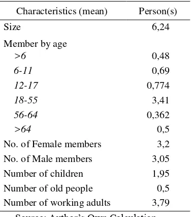
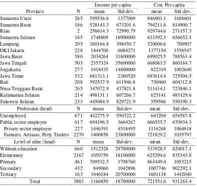
Table 1 summarizes some of the main characteristics of the household in our sample in 2000. In Table 2, we summarize income per head as well as consumption per head according to provinces, employment of household head and level of education of household head.
RESULTS AND ANALYSIS
1. Base model
Before we proceed with our estimations, we need to determine which method is best suited for our data. We used the Hausmann test in order to specify the type of model to be used. The test concluded that the null
hypothesis can be rejected and that the fixed effects are to be preferred to the random effects. Consequently, only variables which vary in time are included in the model.
Table 1. The Main Characteristics of the Sample Households
Characteristics (mean) Person(s)
Size 6,24
Member by age
>6 0,48
6-11 0,69
12-17 0,774
18-55 3,41
56-64 0,362
>64 0,5
No. of Female members 3,2
No. of Male members 3,05
Number of children 1,95
Number of old people 0,5
Number of working adults 3,79
Source: Author’s Own Calculation
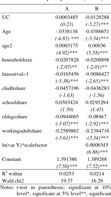
The results of our estimation are reported in table 3. In model A, we regress the growth rate of consumption to our detrended uncertainty variable as well as some variables which are supposed to influence consumption growth rate, using the fixed-effects method. The result of the regression as presented in column A shows that the uncertainty variable is positively correlated with the growth rate of consumption. However the coefficient is not significant thus rejecting the hypothesis of precautionary motive among Indonesian household. As for other variables, most of the coefficients are strongly significant.
In model B, we took into account the fact
that the “poor” may react differently than the “rich” to an increase in uncertainty by
introducing a scaling factor into the equation.
The “rich” who are not financially constrained
uncertainty on the growth rate of consumption will decrease with an increase in the level of wealth of the household.
The results in column B shows that uncertainty is significantly correlated with the growth rate of consumption. Nevertheless the sign is in contrary to what is expected. The coefficient for uncertainty is found to be negatively correlated with the growth rate of consumption per capita which result signifies that in the face of uncertainty, Indonesian
households will increase their current consumption to the detriment of their future consumption. In other words, they do not constitute any precautionary savings to face an increase in uncertainty. As for the variable that captures the effect of wealth, we can see that even though it is significant the sign is in contrary to what is expected. The wealthier is the households, the less they will reduce their present consumption to the detriment of their future consumption. To put it differently, it is Table 2. Income per capita and Consumption per capita According to Province, Employment and
Level of Education
Income per capita Con. Per capita
Province N mean Std-dev. mean Std-dev.
Sumatera Utara 265 599536.6 1377069 846901.1 1688601
Sumatera Barat 186 528143.3 673201.6 794211.8 814900.7
Riau 2 256614.3 72990.79 929744.6 271157.3
Sumatera Selatan 185 1748809 18900000 633392.3 656652.1
Lampung 205 360164.8 398450.7 520606.6 700907
DKI Jakarta 228 1444700 6084271 1377154 1558547
Jawa Barat 580 2034264 31800000 699025.5 788563.4
Jawa Tengah 503 2357324 35600000 668063.5 860184.7
Jogjakarta 277 1418435 14800000 822319 1002640
Jawa Timur 532 681313.1 2360520 693614.4 725504.5
Bali 208 592537.9 611946.8 730460 604312.8
Nusa Tenggara Barat 265 347072.9 437821.8 511414.1 723846.1
Kalimantan Selatan 214 498131.1 607266.7 625141 483129.6
Sulawesi Selatan 233 445084.9 829721.9 559586 550190.3
Profession (head) N mean Std-dev. mean Std-dev.
Unemployed 671 442275.9 950322.2 643204 654587.8
Public sector employee 617 694196.5 3664267 666555.7 670934.3
Private sector employee 227 1446391 4518495 1116268 1064818
Farmers, Artisans, Petty Traders 2270 1400858 23800000 721829.2 1035797
Level of educ (head) N mean Std-dev. mean Std-dev.
Without education 660 1512528 29700000 533928.5 820017.1
Elementary 2167 1050759 18100000 625294.6 835343.8
Primary 461 709532.5 1798760 863449.4 1053215
Secondary 432 849060 1042896 1007746 902292.1
Tertiary 163 3446184 20700000 1601118 1442040
Total 3883 1166850 18700000 721551.6 931263.4
Journal of Indonesian Economy and Business May 228
the “rich” who tends to save more when faced
with uncertainty.
Table 3. Dependant Variable: The Growth Rate of Consumption per Head (lnC)
A B
UC
0.0003485
(0.23)
-0.0129288
(-5.27)***
Age -.0338138
(-4.85) ***
-0.0386651
(-5.54)***
age2 0.0003175
(4.92)***
0.00036
(5.58)***
householdsize -0.0207828
(-2.07)**
-0.0200898
(-2.01)**
lnassetval~1 -0.0165456
(-5.38)***
-0.0086427
(-2.65)***
chidlrshare -0.0457196
(-1.63)
-0.0436283
(-1.56)
schoolshare 0.0303424
(1.50)
0.0293294
(1.45)
oldageshare -0.0944665
(-3.07)***
-0.08947
(-2.92)***
workingadultshare -0.2589862
(-3.61)***
-0.2384716
-(3.34)***
ln(var Y)*scalefactor 0.0008545
(6.88)***
Constant 1.391386
(7.50)***
1.389268
(7.52)***
R2 within 0.0253 0.0214 Wald chi2 19.37 16.29 Notes: t-test in parentheses; significant at 10%
level*, significant at 5% level**, significant at 1% level***.
Source: Processed Data
Based on the results obtained from the estimation of these 2 models, we may conclude that Indonesian households do not have precautionary saving motives. Nevertheless several explanations could be brought forward as to why the growth of consumption and uncertainty is found either to be non-correlated (column A) or negatively correlated (column B). Firstly, the variable used in order to represent uncertainty may not be the most appropriate one. In fact, in the literature, several other methods have been
used in order to come up with the best measure of uncertainty. However, in our case, the choice of method that can be used is somehow constrained by the nature of our data. Secondly, Indonesian households may react to an increase in uncertainty by decreasing only certain type of consumption. Certain expenses are considered as incom-pressible. For example, consumers may not be willing to decrease the amount of their children education expenses of their rents even though they anticipate that their future income will become more risky. If we regress the uncertainty variable to the growth of the total consumption, we may not get a significant correlation between these two variables since, at the same time, there will be some expenses which will be held constant and some others which will be reduced. Thirdly, there may be other types of support mechanism available to the Indonesian households which are not observable by the researchers. The existence of such mechanisms is quite frequent in the developing countries given the social structure of the society. By relying on these measures, households won’t have to reduce their consumption in order to increase their precautionary saving to face uncertainty.
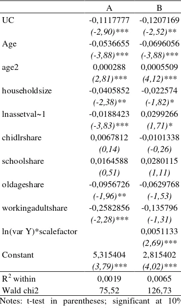
2. Endogeneity problem
It is important to note that the use of the variance of income as a measure of uncer-tainty may lead to the problem of endo-geneity5. Indeed, it is impossible to perfectly measure income notably due to the existence
of what is termed as “measuring error” in the
period lagged of socio-demographic variables as instruments for our uncertainty variable.
The results of our estimation using the instrumental variables method are reported in table 4. Again we estimated two equations: one without controlling for the effects of wealth and another which control for the effect.
Table 4. Dependant Variable : The Growth Rate of Consumption per Head (lnC)
A B
UC
-0,1117777
(-2,90)***
-0,1207169
(-2,52)**
Age -0,0536655
(-3,88)***
-0,0696056
(-3,88)***
age2 0,000288
(2,81)***
0,0005509
(4,12)***
householdsize -0,0405852
(-2,38)**
-0,022574
(-1,82)*
lnassetval~1 -0,0188423
(-3,83)***
0,0299266
(1,71)*
chidlrshare 0,0067812
(0,14)
-0,0101338
(-0,26)
schoolshare 0,0164588
(0,51)
0,0280115
(1,11)
oldageshare -0,0956726
(-1,96)**
-0,0629768
(-1,53)
workingadultshare -0,2582856
(-2,28)***
-0,135796
(-1,31)
ln(var Y)*scalefactor 0,0051133
(2,69)***
Constant 5,315404
(3,79)***
2,815402
(4,02)***
R2 within 0,0019 0,0065 Wald chi2 75,52 126,73 Notes: t-test in parentheses; significant at 10%
level*, significant at 5% level**, significant at 1% level***.
Source: Processed Data
Our regressions show that when the effect of wealth is not controlled for, uncertainty is negatively significantly correlated with the growth rate of consumption per capita (column A). The negative sign of the
uncer-tainty coefficient suggests that Indonesian households do not constitute any precau-tionary saving. In column B, we reported the results of our estimation after controlling for the wealth effect. Again, our results point to the conclusion that Indonesian households do not constitute any precautionary saving in order to face uncertainty. The uncertainty variable is found to be negatively and significantly correlated with the growth rate of consumption per capita. As for the interaction variable that is used to differentiate the effects of uncertainty on the « rich » and the « poor », even though the coefficient is found to be significant, it is not of the expected sign.
CONCLUSION
The main objective of this study is to analyze the behavior of Indonesian household
within a risky environment. We’re interested
in knowing whether uncertainty has a negative impact on the consumption of Indonesian households. This is important particularly in terms of policy implications. If households accumulate more wealth due to uncertainty, policies for reducing uncertainty would reduce precautionary saving and stimulate con-sumption, all factors being equal. Besides, due to precautionary saving, individual households will have to sacrifice a portion of their normal consumption. This will then have an adverse effect on their future well being particularly if the expenses sacrificed concerned the education of their children or their investment in productive materials.
Journal of Indonesian Economy and Business May 230
we may also conclude that Indonesian households rely mostly on informal mecha-nisms in order to face uncertainty. However it is important to emphasize the fact that Indonesia is a country which is developing rapidly. And as the country develops, the structure of its society too may change and it is only a matter of time before it resembles the one that prevails in the developed countries. In such circumstances, social security mecha-nisms which are based mainly on generational and communal solidarity may progressively disappear. And if nothing is done in improving the existing social security system, in case of a shock a large majority of the population will be left without anything to fall back on.
ENDNOTES
1. There are a number of functional forms that can be used in order to capture the impact of uncertainty on consumption. Caroll (1992) showed that a consumption function is concave (which is one of the two conditions required in order to capture the precautionary saving motive) if the utility function used is derived from the family of Hyperbolic Absolute Risk Aversion (HARA) function. Such functions satisfy the following condition
0 2
2 2
3 3
k w
w u w
w u w
w u
In the literature, the two most used utility functions are the Constant Absolute Risk Aversion (CARA) function (where k = 1) and the Constant Relative Risk Aversion (CRRA) function (where k ¿1).
2. The fourth wave of the Indonesia Family Life Survey (IFLS4) was designed between February and September 2007. However, the data will be ready for public viewing by early spring 2009
3. We used 0.5 for children under the age of 7 and 0.8 for older children and senior citizens.
4. Assuming particular processes for income, Carroll (1994) shows that consumers with certain prudence and impatience patterns have a desired wealth income ratio. Bellow this target, prudence dominates and consumers will save; but above, impatience will lead households to dissave, i. e., to use up their wealth surplus.
5. The Nakamura-Nakamura test used to detect the problem of endogeneity reveal that effectively our measure of uncertainty is endogenous.
REFERENCES
Albaran, P., 2000. ‘Income Uncertainty and
Precautionary Saving: Evidence from Household Rotating Panel Data’. CEMFI Workong Paper Series, Working Paper No. 008.
Banks, J., Blundell, R., & Brugiavini, A.,
1999. ‘Risk Pooling, Precautionary Saving and Consumption Growth’. The Institute for Fiscal Studies Working Paper Series, Working Paper No. W99/19.
Bauer, P.T., & Paish, F.W., 1952. ‘The Reduction of Fluctuations in the Incomes
of Primary Producers’. Economic Journal, 62(248), 750-780.
Blundell, R., & Stoker, T., 1998. ‘Consump
-tion and the Timing of Income Risk’.
European Economic Review, 43(3), 475-507.
Browning, M., & Lusardi, A., 1996. ‘House -hold Saving: Micro Theories and Micro
Facts’. Journal of Economic Literature, 34, 1797-1855.
Caballero, R., 1991. ‘Earning Uncertainty and
Aggregate Wealth Accumulation’. Ame-rican Economic Review, 81, 859-871.
Evi-dence’. Brookings Papers Economic .Activity, 1992 2, 61-156.
Carroll, C.D., 1994. ‘How Does Future Income Affect Current Consumption?’.
Quarterly Journal of Economics, 109(1),
111−147.
Carroll, C.D., 2001. ‘A Theory of the Consumption Function, With and Without the Liquidity Constraints, The Journal of Economic Perspectives, 15 (3), 23-45. Carroll, C.D., & Samwick, A.A., 1998. ‘How
Important is Precautionary Saving’.
Review of Economics and Statistics, 80(3): pp. 410-19, August 1998..
Carroll, C., Dynan, K., & Krane, S., 2003.
‘Unemployment Risk and Precautionary
Wealth: Evidence from Households Balance Sheets’. Review of Economics and Statistics, 85(3), 586-604.
Dardoni, V., 1991. ‘Precautionary Savings Under Income Uncertainty: A Cross
Section Analysis’. Applied Economics, 23, 153-160.
Deaton, A. 1992. Understanding Consump-tion, Oxford, Clarendon Press.
Dynan, K.E., 1993. ‘How Prudent are Con
-sumers?’. The Journal of Political Eco-nomy, 101(6), 1104-1113.
Fisher, M.R., 1956. ‘Explorations in Saving
Behaviour’. Oxford University Institute of Statistics Bulletin, 18, 201-277.
Friedman, M. 1957. A Theory of the Consumption Function, Princeton, Princeton University Press.
Guariglia, A., 1998. Understanding Saving Behavior in the UK: Evidence from the BHPS, Mimeo, University of Essex. Guiso, L., Jappelli, T., & Terlizzese, D., 1992.
‘Earnings Uncertainty and Precautionary Saving’. Journal of Monetary Economics, 30, 307-337.
Kazarosian, M., 1997. ‘Precautionary Saving -
A Panel Study’. Review of Economics and Statistics, 79, 241-247.
Kennickell, A., & Lusardi, A., 2004.
‘Disentagling the Importance of
Precautionary Saving Motive. NBER Working Paper Series, Working Paper No W10888.
Kimball, M.S., 1990. ‘Precautionary Saving in the Small and in the Large.’
Econometrica, 58, 53-73.
Kuehlwein, M., 1991. ‘A Test for the Presence of Precautionary Saving’. Economics Letters, 37, 471-475.
Leland, H.E., 1968. ‘Saving and Uncertainty:
The Precautionary Demand for Saving’. Quarterly Journal of Economics, 82, 465-473.
Lusardi, A., 1998. ‘On the Importance of Precautionary Saving’. American Economic Review, 88(2), 449-53.
Lusardi, A., 2000. Precautionary Saving and the Accumulation of Wealth, Mimeo, University of Chicago.
Miller, B.L., 1976. The Effect on Optimal Consumption of Increased Uncertainty in Labor Income in the Multiperiod Case. Journal of Economic Theory, 13(5):154-167.
Merrigan, P., & Normandin, M., 1996.
‘Precautionary Saving Motives: An
Assessment from UK Time Series of Cross-Sections’. Economic Journal, 106, 1193-1208.
Sibley, D.S., 1975. ‘Permanent and Transitory Income Effects in a Model of Optimal Consumption with Wage Income
Uncertainty’. Journal of Economic Theory, 11, 68-82.
Skinner, J., 1987. ‘Risky Income, Life Cycle Consumption and Precautionary Savings’.
NBER Working Paper Series, Working Paper No. 2336.
Zeldes, S. P., 1989. ‘Consumption and
Liquidity Constraint: An Empirical