Volume 26, Number 2, 2011, 235 – 265
ACCOUNTING FUNDAMENTALS AND VARIATIONS OF STOCK
PRICE: FORWARD
LOOKING INFORMATION INDUCEMENT
Sumiyana1
Gadjah Mada University ([email protected])
ABSTRACT
This study investigates a permanent issue about low association between accounting fundamentals and variations of stock prices. It induces not only historical accounting fundamentals, but also forward looking information. Investors consider forward looking information that enables them to predict potential future cash flow, increase predictive power, lessen mispricing error, increase information content and drives future price equilibrium. The accounting fundamentals are earnings yield, book value, profitability, growth opportunities and discount rate or they could be called as five-related-cash flow factors. The forward looking information are expected earnings and expected growth opportunities. This study suggests that model inducing forward looking information could improve association degree between accounting fundamentals and the movements of stock prices. In other words, they have higher value relevance than not by inducing. Finally, this study concludes that inducing forward looking information could predict stock price accurately and reduce stock price deviations from their fundamental value. It also implies that trading strategies should realize to firm’s future rational expectations.
Keywords: earnings yield, book value, profitability, growth opportunities, discount rate, accounting fundamentals, forward looking, value relevance
INTRODUCTION
Permanent issue in accounting is the relationship between accounting information and stock price movements. It is triggered by the objectives of financial reporting (FASB, 1978) stated that financial reporting must presents information for both investors and potential investors to estimate future cash flow. Consequently, it requires close associa-tion between fundamental firm value and its changes with stock price variations. The objective of this study is to evaluate this
association by designing new better model, especially to estimate the value relevance of firms’ fundamental value.
Chen and Zhang (2007) present theory and empirical evidences that stock return is a function of accounting fundamentals. They indicate that firm equity value contains future potential earnings and growth opportunities. Lev (1989), Lo and Lys (2000), and Kothari (2001) have studied the association between stock return and fundamental accounting information and found that it is contradictory.
They denote that the inconsistent association due to (1) weak relationship between earnings and stock price variations, represented by adj-R2 less than 10% (Chen and Zhang, 2007), and (2) linearity relationship between accounting information and future cash flow, with scala-bility of equity capital investment (Ohlson, 1995, Feltham and Ohlson, 1995, 1996, Zhang, 2000, and Chen and Zhang, 2007).
This study focuses on designing new return model by inducing forward looking information to improve association degree between accounting fundamentals and stock price variations. Zhang (2000) and Chen and Zhang (2007) models include historical accounting data or backward looking perspec-tive. Based on that model, this study induces expected future earnings yield and growth opportunities or has forward looking informa-tion. It has some advantages. They are able to achieve value optimization (Shaw, 2007), give superiority to future information (Lee and Yan, 2003), improve model accuracy (Chen, Yee, and Yoo, 2004), reduce future uncer-tainty (Giannnoni, 2008), and reduce stock price fluctuation (Brock, Dindo, and Hommes, 2006). This study is different from Copeland et al. (2004), and Liu and Thomas (2000). Both studies focus on expected future earnings only. Meanwhile, it is also different from Weiss, Naik and Tsai (2008) that induce short-run asset capacity.
This study investigates return model by employing several capital markets that are Asia, Australia and US countries. Although all these countries are not comparable in eco-nomic progress and capital market efficiency form, this study blends them. This blending is based upon market-wide regime shifting behavior concept (Ho and Sequeira, 2007). This concept recommends that the association between accounting fundamentals and stock price movements is only based on earnings and firm book value. It also suggests that highly stock price movement respons to highly earnings level and vice versa. It could be
concluded that this reaction do not consider market efficiency form.
This study is based on two assumptions. Firstly, stock markets in selected countries are within comparable efficiency level. Stock price variations at all stock markets acts in the same market-wide regime behavior and depends on equity book value and earnings (Ho and Sequeira, 2007). Secondly, cost of interest represents opportunity cost for each firm. It describes that every fund was managed in order to maximize assets usability. This refers to that management always behaves rationally.
Research Objectives
The main objective of this study is to construct new return model and examine it to obtain better association degree. It also inves-tigates consistent direction of each construct association within the return model. The new return model induces forward looking infor-mation which is not potential expected earnings (Weiss, Naik and Tsai, 2008) or multiple earnings only (Liu, Nissim and Thomas, 2001), but it also induces both of expected future earnings and growth oppor-tunities. Finally, this study examines previ-ously designed model and compares with the new one.
Research Contribution
Second, by inducing forward looking information, this model is expected to be more realistic and closer to economic perspective. It means that, in accordance with forward looking theory, the firm should make rational decision to manage its assets to generate future cash flow. The firm must choose future investments which give positive contribution to future cash flow. Future cash flow affects earnings and its change. It refers to earnings capitalization model. Third, this new model becomes more accurate and better instrument to predict future cash flow. It is useful for investors to estimate future potential gains by extracting forward looking information (Weiss, Naik and Tsai, 2008). Its accuracy is supported by multiple value drivers (Liu, Nissim and Thomas, 2001). Multiple value drivers increase model accuracy as long as they have information synchronicity to increase value relevance. Last, this study has valuable contribution by creating new return model with higher association degree. It is showed by adj-R2 which is higher than previous models.
Research Benefits
This study is beneficial to investors and managements. From investor’s point of view, this study offers more accurate, comprehen-sive parameter to predict future cash flow (SFAC No. 1, FASB, 1978). This is related to the relationship of fundamental accounting data and its change with stock price. Account-ing information becomes more useful when presented in financial statements (SFAC No. 5, para. 24, FASB, 1984).
From management’s point of view, this study gives more incentive for managements to manage more rationally their future invest-ments giving positive contribution to firm equity value. Managements and investors should perceive closely the association between accounting information and stock price. From accounting literature point of view, this study becomes a trigger to further
studies, especially to develop new models to achieve higher degree of association.
The remaining manuscript is organized as follows. Section 2 describes the development of theoretical return model and hypothesis for each model. Section 3 illustrates empirical research design and research methods. Section 4 discusses the results of empirical examina-tions. And section 5 depicts research conclu-sions, limitations and consequences for further studies.
LITERATURE REVIEW, MODEL AND HYPOTHESES DEVELOPMENT
Earnings Yield and Book value
Model that associates earnings and book value with stock market value or return is developed on classical concepts basis. The point is the usage of accounting information to evaluate firm equity value, market efficiency, and forecasting analysis. This concept refers to Ohlson (1995). This model formulates that firm equity value comes from book value and expected value of future residual earnings. The expected value can be calculated from current discounted value of potential assets. Every new wealth acquired comes from invested assets and being reflected in firm book value. Then, firm book value is reflected in stock price.
Model of Ohlson (1995) indicates linear information dynamic between book value and expected residual earnings with stock price. This model is followed by next studies. Lo and Lys (2000), and Myers (1999) for the first time implemented clean surplus theory. It outlines that end year book value equals to beginning year book value added by current year earnings and subtracted dividend paid. Model of Lundholm (1995) formulates that firm market value equals to equity capital invested plus discounted future residual earnings.
equity value and to determine either earnings or firm market value. Lo and Lys (2000) offer new hypothetical concepts that firm equity value is a function of discounted future earnings and dividend. Dechow, Hutton, and Sloan (1999) evaluate capital rate of return based on residual earnings, while Frankel and Lee (1999) add investors expectation of minimum profitability. Beaver (1999), Hand (2001), and Myers (1999) confirm that firm market value is a function of book value and earnings, in accordance with concept of Ohlson (1995). However, the three researches recommend other information to increase association degree of return model. Ohlson (2001) criticize his former concept by describing other information to increase degree of association between book value and earnings with firm market value. Danielson and Dowdell (2001) and Aboody, Hughes and Liu (2001) specify the other information with growth rate and reasonable expectation of future earnings.
Other studies constantly use model of Ohlson (1995) without criticizing book value and earnings within the model. Feltham and Ohlson (1995; 1996) emphasize that the association between book value and earnings is asymptotic; it may be affected by other information and conservatism in depreciation. Burgstahler and Dichev (1997), under the same model, add concept of assets book value and liabilities to explain firm market value better. Liu and Thomas (2000), and Liu, Nissim and Thomas (2001) add multiple factors into clean surplus model, either earnings dis-aggregation or other book value and earnings related measures.
Collins, Maydew, and Weiss (1997), Lev and Zarowin (1999), and Francis and Schipper (1999) outline that value relevance between book value and earnings with stock market value or return may be preserved. Abarbanell and Bushee (1997) and Penmann (1998) specifically that more accounting information result in better degree of association. Both
studies earnings quality improve degree of association. Collins, Pincus, and Xie (1999) argue similarly and confirm the association between book value and earnings with stock market value by eliminating losing firms.
Bradshaw, Richardson and Sloan (2006) modify clean surplus model by adding future financing activity. Cohen and Lys (2006) and Weiss, Naik and Tsai (2008) add expected value of future potential earnings into return model. Chen and Zhang (2007) modify their model without discarding book value and earnings. This research, in order to increase degree of association, adds external environ-ment factors which may multiply degree of association.
Past researches have correlated book value and earnings with firm market value. Rao and Litzenberger (1971), and Litzenberger and Rao (1972) formulate that firm market value is a function of book value and earnings and adjustable to liabilities and productivity growth. Bao and Bao (1989) indicate that firm equity value is not merely affected by earning, but also by expected earnings, earnings stan-dard deviation and earnings growth. Beaver, Lambert and Morse (1980), Collins, Kothari and Rayburn (1987), Easton and Harris (1991) conclude that book value and earnings have better degree of association when the earnings are ranked. Earnings and their changes are deflated by stock market value. Warfield and Wild (1992) examine further than Easton and Harris (1991) and replace the deflating factor with previous year stock market value.
ForwardLooking Information
accounting information which are comparable within a set of information (Heijdra and Ploeg, 2002). The benefit and objective is to obtain more effective information set for decision making. It is a more universal instrument to investigate the implications of new policies for it measures asymptotic variance. The value relevance can be either in short-term or long-term.
Another advantage of forward looking information is its transparency and predictive power (Zarb, 2007; Fay, 2009). Shaw (2007) indicates that forward looking information is able to predict cash inflow and potential future cash flow better than backward looking information. Therefore, it can be used for fore-casting and maximizing technique. Beretta and Bozzolan (2006), and Chen, Yee and Yoo (2004) conclude that inducing forward looking information increase predictive power and lessen forecasting error. Dikolli and Sedatole (2007) conclude that forward looking information of non-main earnings increase information content. Moreover, it brings better indicator for decision making. Giannoni and Woodford (2007) state that forward looking information makes forecasting more efficient within longer period and predict clearly future benefits. Brock, Dindo, and Hommes (2006) conclude that forward looking information drives price equilibrium in the future. Within return model context, it makes return model achieve equilibrium state.
The mapping of accounting researches gives concept to anticipate future reasonable expected values. Beaver, Lambert and Morse (1980) initiate that their research include future earnings change into return model. This study is supported by Lev and Thiagarajan (1993), Abarbanell and Bushee (1997), Brown, Foster, and Noreen (1985), and Cornell and Landsman (1989). Easton and Harris (1991) also perform similar study, with future expected return is deflated by previous year stock price as predictor in return model. Liu and Thomas (2000) give solution that
future earnings and earning shock improve association degree of return model. This model offers more effective model and decrease specifying errors.
Copeland, et al. (2004) confirms that reasonable future expected earnings improve return model. Chen and Zhang (2007) specify that expected earnings, expected future growth rate, and expected discount rate change improve association degree of return model. Weiss, Naik and Tsai (2008) design their own return model by including forward looking information of short-term investment capacity. This study gives stronger degree of associa-tion. Forward looking information included into this model consists of future account receivables, future inventory, future profit margin, and future cost of good sold. It can be concluded that inducing reasonable expected future values improves return model.
Change in Growth Opportunities
Growth opportunities are included into return model according to model of Ohlson (1995). This model complies to clean surplus theory, with premises as follows. (i) Stock market value is based on discounted dividend in which investors take neutral position against risks. (ii) accounting income is pre-determinis-tic value. (iii) In addition, future earnings are stochastic. Future earnings can be calculated by previous consecutive earnings. However, investors may have different respond against minimum or maximum profitability. There-fore, growth opportunities affect earnings or future potential earnings.
on concept of Miller and Modigliani (1961) who concluded that a growing firm is firm with positive capital rate of return. It also means that each asset has lower interest rate than cost of capital.
Liu, Nissim and Thomas (2001), Aboody, Hughes and Liu (2002), and Frankel and Lee (1998) mention that firm intrinsic value is determined by growth and future potential growth. Current growth drives the movement of future residual earnings, while future growth lessens return model errors by improving association degree of return model. Lev and Thiagarajan (1993), Abarbanell and Bushee (1997), and Weiss, Naik and Tsai (2008) indicate that changes in inventory, gross profit, sales, account receivables and the others improve future potential growth of earnings. Growth also improves firm equity value. The study concluded that stock market value is adjustable to that firm’s growth. Danielson and Dowdell (2001) confirm that growing firm has better operation efficiency. Growing firm always has ratio between stock price and book value greater than one. However, investors do not perceive stock return of growing firm higher than those of diminishing firm.
Chen and Zhang (2007) conclude that firm equity value depends on growth opportunities. Growth opportunities are a function of scaled investment and affects future potential growth. The inducement of growth opportunities argues that earnings elements alone are not sufficient to explain. The explanation becomes more comprehensive when external environ-ment, industry and interest rate are included to determine earnings and future earnings.
Change in Discount Rate
Change in discount rate concept is based on model of Ohlson (1995) simplification. This model assumes that investors take neutral position against fixed risks and interest rate. The simplification is modified by Feltham and Ohlson (1995; 1996), and Baginski and
Wahlen (2000) by inducing interest rate because it affects short-term and long-term earnings power. Change of interest rate also affects investor’s perception about earnings power, because interest rate provides certainty of future earnings.
Rao and Litzenberger (1971), and Litzenberger and Rao (1972) posit that firm equity value depends on discounted value of future earnings. This value is affected by pure interest rate. Interest rate changes operation efficiency. Operation efficiency alters earn-ings. Danielson and Dowdell (2001), and Liu, Nissim and Thomas (2001) state that discount rate modifies firm equity value for it changes the growth of assets and capital book value. If weighted interest rate of assets and capital was higher than pure interest rate, the firm may generate earnings. Obtaining new debts or capital can decrease weighted interest rate.
Burgstahler and Dichev (1997) indicate that firm equity value can be increased according to adaptation theory by modifying interest rate, for instance obtaining alternative investment with lower interest rate. Aboody, Hughes and Liu (2002), Frankel and Lee (1998), Zhang (2000) and Chen and Zhang (2007) argue that earnings growth is deter-mined by interest rate. Interest rate serves as adjustment factor for firm operation, by selecting favorable interest rate to make efficient operation.
Model of Equity Value
Earnings play important role to show the firm tendency to grow or to terminate its operation. Valuation model measures the creation of equity capital investment on continuation or termination of firm operation framework (Burgstahler and Dichev, 1997). Equity value model developed by Zhang (2000) and Chen and Zhang (2007) is described as follows.
With Vt is firm equity value financed
during period t, Bt is equity book value,
Et(Xt+1) is future expected earnings, k is
earnings capitalization factor, P is probability of operation termination, C is probability of operation continuation, qt ≡ Xt/Bt-1 is
profitability, based on ROE, period t. and gt is
growth opportunities, Chen and Zhang (2007) formulate equity value as follows.
)
This model (1) formulates that equity value (Vt) is correlated with future expected
earnings (Et(Xt+1), future earnings
capitaliza-tion factor (k), probability to terminate operation (P(qt)), and probability to continue
operation (C(qt)). It indicates that equity value
is equal to current operation (qt) added by
growth value which can be positive or negative (gt). It also indicates that when v
increased, then gt increase along with invested
assets. Increase of v makes discount rate rt to
fall which indicates easier future cash flow. Therefore, firms with gt increase and rt
decrease are firms those are able to generate earnings.
Model of Stock Return with Inducing
ForwardLooking Information
Using model (1) as basis, forward looking model for expected earnings is as follows.
⎥
The next is inducing forward looking informa-tion of expected profitability into model (3) to obtain model (3) as follows.
⎥
Equation (3) infers that stock return is a function of the following factors: (1) earnings yield (Xt/Vt-1), (2) expected earnings (EXt+1/Vt),
(3) change in equity capital (ΔBt/Bt-1), (4)
change in growth opportunities (Δgt), (5)
change in expected growth opportunities (ΔEgt+1), and (6) change in discount rate (Δrt).
Up to this stage, model was developed incrementally, forward looking variables are included into model one by one. Though, actually it can be done mutually exclusive.
Hypothesis Development
EarningsYield Earnings yields (Xt) show
Using mathematical properties from equation (3), the association between earnings yields (Xt/Vt-1) and stock return (Rt) should be
positive. It is caused by
1
is always positive. Therefore, my alternative hypothesis is stated as follows.
HA1: Earnings yield associates positively with
stock return
Expected Earnings Similar to earnings
yield, expected earnings (EXt+1) shows value
which is expected to be generated in the future from end year capital. Expected earnings are normalized by closing value of current capital, so that potential future earnings growth is shown. Inducing expected earnings is based on forward looking concept which states that reasonable future expected earnings influences positively the movement of stock price or certain measure (Burgstahler and Dichev, 1997; Cohen and Lys, 2006; Weiss, Naik and Tsai, 2008; Chen and Zhang, 2007; Ohlson, 1995; Feltham and Ohlson, 1995; Feltham and Ohlson, 1996; and Aboody, Hughes and Liu, 2001).
The influent mechanism is equal to earnings yield, so that the association between expected earnings (EXt+1/Vt) and stock return
is positive. It is also caused by
t
summarize alternative hypothesis statement as follows.
HA2: The change in expected earnings yield
associates positively with stock return
Change in EquityCapital The change in
equity capital is center of firm value measurement. It is measured by ΔBt/Bt-1 which
is change in current equity value divided by beginning value of current equity. Because of
ΔBt/Bt-1=v[ΔBt/Vt-1], the change of equity
value increases as equity capital does, then reflected in stock return. In other words, the change of stock return is in accordance with the change of earnings after denominated by opening value of current capital (Vt-1).
Therefore, v is always positive and greater than zero. It means that change in equity capital associates positively with stock return (Rao and Litzenberger, 1971; Litzenberger and Rao, 1972; Bao and Bao, 1989; Burgstahler and Dichev, 1997; Collins, Pincus and Xie, 1999; Collins, Kothari and Rayburn, 1987; Cohen and Lys, 2006; Liu and Thomas, 2000; Liu, Nissim and Thomas, 2001; Weiss, Naik and Tsai, 2008; Chen and Zhang, 2007; Ohlson, 1995; Feltham and Ohlson, 1995; Feltham and Ohlson, 1996; Bradshaw, Richardson and Sloan, 2006; Abarbanell and Bushee, 1997; Lev and Thiagarajan, 1993; Penman, 1998; Francis and Schipper, 1999; Danielson and Dowdell, 2001; Aboody, Hughes and Liu, 2001; Easton and Harris, 1991; and Warfield and Wild, 1992).
Using mathematical properties from equation (3), the association between change in equity capital and stock return should be positive. It is caused by
1
dRt/dBt should be positive and greater than
zero. It is summarized as alternative hypothe-sis as follows.
HA3: Change in equity capital associates
positively with stock return
Change in Growth Opportunities Future
equity value depends on change in growth opportunities (Δgt). Stock return depends on
whether a firm grows or not. If a firm grown, it increases its equity value and simultaneously stock return increases. This growth concept is supported by growth adjustment process using Bt-1/Vt-1. Because of a growing firm is able to
indicates that assets grow in different pace than equity value. Therefore, growth oppor-tunities (Δgt), after being adjusted by Bt-1/Vt-1
associates positively with stock return (Rao and Litzenberger, 1971; Litzenberger and Rao, 1972; Bao and Bao, 1989; Weiss, Naik and Tsai, 2008; Ohlson, 1995; Abarbanell and Bushee, 1997; Lev and Thiagarajan, 1993; Danielson and Dowdell, 2001; and Aboody, Hughes and Liu, 2001). The alternative hypo-thesis is stated as follows.
HA4: Change in growth opportunities
associ-ates positively with stock return
Change in Expected Growth Oppor-tunities Future firm equity value is influenced by the change in expected growth opportuni-ties (ΔEgt+1). Its explanation is equal to growth
opportunities. The association between change in expected growth opportunities (ΔEgt+1) is
also positive (Rao and Litzenberger, 1971; Litzenberger and Rao, 1972; Bao and Bao, 1989; Weiss, Naik and Tsai, 2008; Ohlson, 1995; Abarbanell and Bushee, 1997; Lev and Thiagarajan, 1993; Danielson and Dowdell, 2001; and Aboody, Hughes and Liu, 2001). Similarly, alternative hypothesis is stated as follows.
HA5: Change in expected growth opportunities
associates positively with stock return
Change in Discount Rate Discount rate
shows future cash flow valued by cost of capital. The change in discount rate (Δrt)
affects future cash flow then modifies stock return in turn. The higher discount rate, the lower future cash flow and vice versa. It means that change in discount rate associate negatively with stock price variations (Rao and Litzenberger, 1971; Litzenberger and Rao, 1972; Burgstahler and Dichev, 1997; Liu, Nissim and Thomas, 2001; Chen and Zhang, 2007; Feltham and Ohlson, 1995; Feltham and Ohlson, 1996; Danielson and Dowdell, 2001; and Easton and Harris, 1991).
Using mathematical properties from equation (3), the coefficient of Δrt should be
negative. It is caused by
1
unit of investment, but because of
k
should be less than zero. It is sum-marized in the following hypothesis statement.
HA6: Change in discount rate associates
negatively with stock return
RESEARCH METHOD
Population and Sample
All return-related-cash flow factors in this study (earnings yield, expected earnings yield, change in equity, and change in growth opportunities and its expected value) are obtained from financial statements. Expected data or prospectus for next year is included within notes of financial statements. All data are available at OSIRIS database. The change of discount rate data are obtained from central bank official website of each country, even though financial statements usually contain long-term debts or long term interest rate. The change of discount rate is proxies by long-term obligation interest rate from central bank of each country. Then, this study extracts stock price and return for each firm at each stock market directly.
movement as respond to accounting informa-tion should be equal.
Sampling Methods
This study uses purposive sampling, the sample is obtained under certain criteria. The criteria are as follows. First, firms are in manufacture and trading sectors, eliminating financial and banking sectors. This study eliminates financial and banking sectors because they are regulated tightly. Second, opening and closing equity book value must be positive (Bit-1>0; Bit>0). Firms with
nega-tive equity book value tend to go bankruptcy. Third, accounting information and its expecta-tion or prospectus is available. They are required for inducing forward looking infor-mation. Fourth, firm stocks are traded actively. Sleeping stocks would disturb conclusion validity.
Variables Measurement and Examination
This study designs model to improve model of Chen and Zhang (2007) by inducing forward looking information. Briefly, this study is carried out in consecutive stages as follows. First, examine using model of Chen and Zhang (2007). Second, examine by our newly developed model by inducing backward looking and forward looking information. Next, this study compares the results of both previous examinations.
The first examination is using model of Chen and Zhang (2007). It uses linear regression examination based on model as follows.
With Rit is annual stock return for firm i during
period t, measured since the first day of opening year period t-1 until one day after financial statement publication or, if any, earnings announcement period t; xit is earnings
firm i during period t, calculated by earnings
acquired by common stock holders during period t (Xit) divided by equity market value
during opening of current period (Vit-1);
1
profitability firm i during period t, deflated by equity book value during opening of current period and profitability calculated using formula qit=Xit/bit-1;
equity capital or proportional change in equity book value for firm i during period t, adjusted by one minus ratio book value and market value during current period. This adjustment is needed to balance accounting book value and market value; Δgˆit =(git−git−1)Bit−1/Vit−1 is change in growth opportunities firm i during period t; Δrˆit =(rit −rit−1)Bit−1/Vit−1 is change in discount rate during period t; α, β, γ, δ, ω and ϕ are regression coefficient; and eit is
residual.
The second examination is inducing expected earnings, using model as follows.
it earnings firm i during period t+1 calculated by dividing following period expected earnings (EXit+1) with current period equity book value
(Vt).
The third examination is inducing expected growth opportunities into model (4), so that the result is as following model.
Until model (6) inducing forward looking variables is performed mutually exclusive. After that, all forward looking variables are induced simultaneously using model as follows.
Linearity examination is conducted for each model. The reason is that all models are linear regression and require freedom of normality, heteroscedasticity, and multicolli-nearity. As Gujarati (2003) states that linear regression model must control its residual errors to prevent bias.
Sensitivity Examination
Sensitivity examination for cross-sectional data which has been examined by model (4) until (7) is performed by sample arrangement into various partitions. Partitioning criteria are ratio between equity book value and stock market value. This examination is aimed to show model consistency within various market levels. Consistency is also expected to be shown at various market changes. Our return model examines consistency against system-atic risks, and not yet against idiosyncrsystem-atic risks. The examination is carried out by splitting sample into quintiles or deciles according to ratio of book value and market value.
Robustness Examination
Beside sensitivity examination, this study also examines the model robustness. The objective is to infer the consistency of return model not only considering systematic risks but also idiosyncratic risks. Robustness exami-nation employs abnormal return. Idiosyncratic risks are verified when fundamental account-ing information was related to abnormal return. In other words, it also anticipates investor’s overreaction against accounting information. In this study, abnormal return
refers to part of abnormal return which can not be explained by main factors as explained in model of Fama and French (1992, 1993, dan 1995). This model formulates that return as a factor of ME (market equity) which is market based measurement, and BE/ME (book-to-market) which is ratio between book value and market value of each share. Therefore, model of Fama and French (1992, 1993, dan 1995) formulation is as follows.
it
Model (8) results residual error, noted as eit. It may be used as abnormal return indicator
(Fama and MacBeth, 1973), and serves to examine incremental explanatory power (Chen and Zhang, 2007). It is expected to explain additional explanatory power of all independ-ent variables in all models. Fundamindepend-ental accounting information should able to explain stock price movements or has relevance value with earnings.
ANALYSIS, DISCUSSION AND FINDINGS
This section describes data analysis, discussion and research findings. It starts with descriptive statistics, analysis, discussion and ends with research findings. Descriptive statistics initiate this description.
Descriptive Statistics
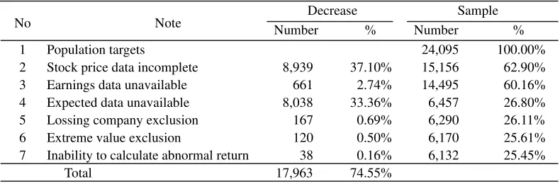
(0.69%) are caused by negative earnings. Fifth, 120 (0.50%) are due to extreme data exclusion. Last, 38 (0.16%) are caused by abnormal return that cannot be calculated using model of Fama and French (1992, 1993, and 1995).
Final sample has fulfilled all required criteria. This study cannot obtain firms with negative book value, because their stock price data is incomplete. Therefore, the criterion which excludes firms having negative book value is automatically accomplished. The acquired data and the exclusion are presented in Table 1 as follows.
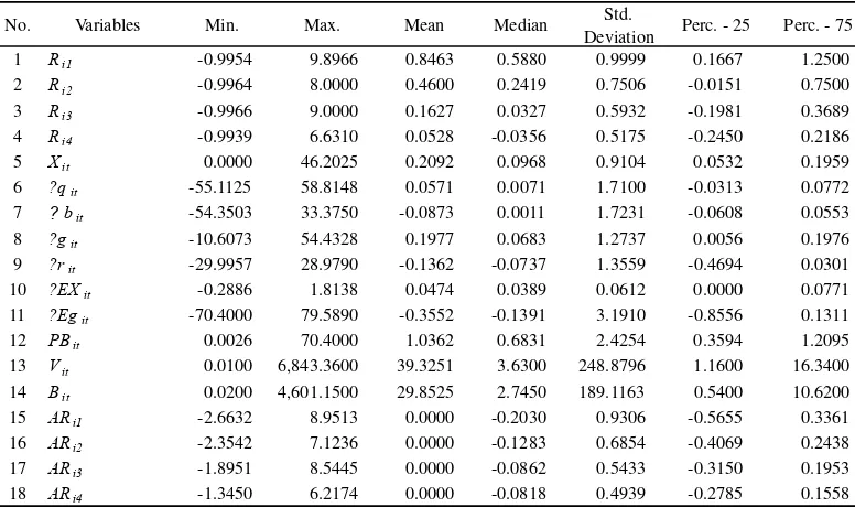
From sample, this study analyzes to examine data initial tendency. The result of descriptive statistics is shown in Table 2. It can be inferred as follows. Return for one year period (Ri1) is 0.8463. then, it degrades during
the following periods, for return (Ri4) becomes
0.0528. The decrease occurs in all level of percentile 25 (from 0.1667 to -0.2450) and percentile 75 (from 1.2500 to 0.2186). It indicates that firm market value in longer period becomes closer to its intrinsic value. With this proximity, fundamental accounting information is expected to be reflected in firm market value.
Since earnings data used in this study are earnings after tax (xit), it requires firms with
profit. Therefore, the minimum value is 0.0000. Mean value is 0.2092, median value is 0.0968, and standard deviation is 0.9104. The median value is in the left side of mean. It shows that there are some firms having enormous earnings. However, this condition is not a problem since its standard deviation is less than one. The return data indicates similar tendency. Therefore, the correlation between both variables is possible. The other variables, change of earnings power (Δqit) and change of
growth opportunities (Δgit) also show similar
tendency as earnings. Meanwhile, change of discount rate shows inversed tendency. Such phenomena are expected.
The change of expected earnings may move positively or negatively. Declined predicted firms show negative fluctuation. Expected earnings have minimum value of -0.2886, maximum value of 1. 8138, mean of 0.0474 and median of 0.0389. Standard deviation shows as much as 0.0612 relatively small standard error of estimate. The change of growth opportunities (EΔgit) shows
com-parable tendency. It indicates that all expected values fluctuate in accordance with stock price or return. With such initial indication, the
Table 1 Sample Data
Number % Number %
1 Population targets 24,095 100.00%
2 Stock price data incomplete 8,939 37.10% 15,156 62.90%
3 Earnings data unavailable 661 2.74% 14,495 60.16%
4 Expected data unavailable 8,038 33.36% 6,457 26.80%
5 Lossing company exclusion 167 0.69% 6,290 26.11%
6 Extreme value exclusion 120 0.50% 6,170 25.61%
7 Inability to calculate abnormal return 38 0.16% 6,132 25.45%
Total 17,963 74.55%
No Note
Decrease Sample
association between expected value of accounting information and firm market value is positive. Forward looking information probably associates with stock price or return.
Firm book value (Bit), ratio between
market price and book value (PBit), and stock
market value (Vit) are always positive. This
study eliminates firms with negative book value and having losses. Even though extreme values have been eliminated, maximum values for Bit and Vit still show great numbers. It
especially occurs in developing countries where stock market value deviates from its book value. With mean of 29.8525 and median of 2.7450 Bit is in accordance with stock
market value. Such indication does not disturb model validity. Pattern of such is also shown
by firm intrinsic value (Vit) which is reflected
in closing value of stock market price.
Abnormal return calculated with model of Fama and French (1992; 1993 and 1995) shows mean of 0.0000 for ARi1, ARi2, ARi3, dan
ARi4. It means that estimation of abnormal
return is valid mathematically. The standard deviation of abnormal return becomes smaller over time, from 0.9306 (ARi1) become 0.4939
(ARi4). The standard deviation indicates that
abnormal return fluctuates in the same pattern as firm market value. Abnormal return fluctuation is also similar with return and earnings (xit), change of earnings power (Δqit),
and change of growth opportunities (Δgit).
Such indication supports our hypotheses.
Table 2 Descriptive Statistics
No. Variables Min. Max. Mean Median Std.
Deviation Perc. - 25 Perc. - 75
1 Ri1 -0.9954 9.8966 0.8463 0.5880 0.9999 0.1667 1.2500
2 Ri2 -0.9964 8.0000 0.4600 0.2419 0.7506 -0.0151 0.7500
3 Ri3 -0.9966 9.0000 0.1627 0.0327 0.5932 -0.1981 0.3689
4 Ri4 -0.9939 6.6310 0.0528 -0.0356 0.5175 -0.2450 0.2186
5 Xit 0.0000 46.2025 0.2092 0.0968 0.9104 0.0532 0.1959
6 ?qit -55.1125 58.8148 0.0571 0.0071 1.7100 -0.0313 0.0772
7 ?bit -54.3503 33.3750 -0.0873 0.0011 1.7231 -0.0608 0.0553
8 ?git -10.6073 54.4328 0.1977 0.0683 1.2737 0.0056 0.1976
9 ?rit -29.9957 28.9790 -0.1362 -0.0737 1.3559 -0.4694 0.0301
10 ?EXit -0.2886 1.8138 0.0474 0.0389 0.0612 0.0000 0.0771
11 ?Egit -70.4000 79.5890 -0.3552 -0.1391 3.1910 -0.8556 0.1311
12 PBit 0.0026 70.4000 1.0362 0.6831 2.4254 0.3594 1.2095
13 Vit 0.0100 6,843.3600 39.3251 3.6300 248.8796 1.1600 16.3400
14 Bit 0.0200 4,601.1500 29.8525 2.7450 189.1163 0.5400 10.6200
15 ARi1 -2.6632 8.9513 0.0000 -0.2030 0.9306 -0.5655 0.3361
16 ARi2 -2.3542 7.1236 0.0000 -0.1283 0.6854 -0.4069 0.2438
17 ARi3 -1.8951 8.5445 0.0000 -0.0862 0.5433 -0.3150 0.1953
18 ARi4 -1.3450 6.2174 0.0000 -0.0818 0.4939 -0.2785 0.1558
Notes: Number of observation (N): 6.132. Rit: stock return for firm i during period 1 (1 year), 2 (1 year 3
months), 3 (1 year 6 months), and 4 (1 year 9 months); xit: earnings for firm i during period t; Δqit: change of profitability for firm i during period t; Δbit: change of book value for firm i during period
t; Δgit: change of growth opportunities for firm i during period t; Δrit: change of discount rate during period t;E: abbreviation of Expected value; PBit: ratio between stock market value and book value for firm i during period t; Vit: market value of stock firm i during period t; Bit: book value for firm i during period t; ARit: stock abnormal return for firm i during period 1 (1 year), 2 (1 year 3 months), 3
Basic Model (Chen and Zhang, 2007) Analysis
As first stage, this study examines model of Chen and Zhang (2007), it is henceforth called the basic model (model 4). It constructs five main factors which associate with return. They are earnings (xit), change in firm book
value (Δbit), change in earnings power (Δqit),
change in growth opportunities (Δgit), and
change in discount rate (Δrit). The result
analysis is presented in Table 3 as follows. This basic model examination serves as initial investigation of association between five factors with stock return. The result shows that earnings (xit), firm book value (Δbit), and
growth opportunities (Δgit) are consistently
above 1% confirmed that they associate with stock return for various return specifications (Ri1 until Ri4). This study is failed to confirm
the association between earnings power (Δqit)
with stock return, unlike Chen and Zhang (2007) who confirm it consistently. Meanwhile, change in discount rate (Δrit) is
not consistently confirmed. Therefore, this study concludes that model of Chen and Zhang (2007) is adequately supported except for earnings power. Degree of association shows F-value of 35.5187 and significant at level 1%. This basic model has return type R2 of 2.82% for Ri1, and lower for the others. Its
adj-R2 value is 2.74%.
The result of first stage examination is interesting. Earnings power and change in discount rate are not confirmed their association with stock returns. Even though the basic model is still able to conclude the association between accounting information and return, it is not flexible enough or rigid
because the two variables above were not confirmed. Therefore, this result gives suffi-cient reason for further stage of examination. This study suspects that forward looking information can be induced into model.
Inducing Change in Expected Earnings into Model
This model initiates the inducing of forward looking information as basic model modification. This model, hereafter, is called model 5. The result of model 5 examination is presented in Table 4 as follows.
The result shows that hypothesis HA1 is
supported. It means that earnings yield associates positively with stock price variations. Hypothesis HA3 which states that
change in equity capital associates with stock return is supported. The same thing goes to hypothesis HA4 which states that change in
growth opportunities associates with stock return. The three hypotheses are supported in all return types Ri1 – Ri4. Furthermore, the
result indicates that change in expected earnings associates with return with t-value of 2.5826 and is significant at level 1% for Ri4
type. Therefore, change in expected earnings (ΔExit) associates positively with stock return
or hypothesis HA2 is supported. The
confir-mation in Ri4 returns type because change in
expected earnings is measured annually. Then it associates with stock return which is also in annual measure. This examination cannot confirm hypothesis HA6, that change in
discount rate explain stock price movements. This model 5 has R2 value of 2.82% for Ri1
24
9
Table 3 Basic Model Analysis
Notes: Number of observation (N): 6.132. Rit: stock return for firm i during period 1 (1 year), 2 (1 year 3 months), 3 (1 year 6 months), and 4 (1 year 9
months); xit: earnings for firm i during period t; Δqit: change in profitability for firm i during period t; Δbit: change in book value firm i during period
t; Δgit: change in growth opportunities for firm i during period t; Δrit: change in discount rate during period t; *** significant at level 1%, **
significant at level 5%, * significant at level 10%. Linearity examination for model 4 shows that: (1) Kolmogorov-Smirnov test is not passed with value of 9.036 and p-value 0.000, and Jarque and Berra test is not passed with value of 15,202.42 with chi-square 0.000 which means that the residual is distributed non normally. However, normality examination is ignorable for large data sample (6,132) since it tends to follow centralized limit theorem (Gudjarati, 2003). (2) Glejser’s test shows that all variables are significant above 0.05, with t-value (sig.), xit as much of 0.013(0.989);
Δqit as much of -0.014 (0.989); Δbit as much -0.007 (0.994); Δgit as much of -0.073 (0.942); and Δrit as much of 0.010 (0.992). Therefore, it shows
that all variables are clear from heteroscedasticity problem. (3) Multicollinearity test shows that all variables have VIF around one which means that collinearity between variables is deniable, VIF value for xit is 2.394; Δqit is 1.483; Δbit is 1.664; Δgit is 1.218; and Δrit is 1,010. Detailed correlation
matrix is in additional table as follows.
Additional table:
Variables
Δqit 0.526 ***
Δbit -0.620 *** -0.247 ***
Δgit 0.353 *** -0.004 -0.284 ***
Δrit 0.028 ** -0.007 0.043 *** -0.031 **
ΔEXit 0.007 -0.008 0.014 -0.019 0.058 ***
ΔEgit -0.366 *** -0.154 *** 0.280 *** -0.344 *** 0.117 *** 0.284 ***
Xit Δqit Δbit Δgit Δrit ΔEXit
J
o
urna
l of
Indo
nesi
a
n
Eco
n
omy and Business
Ma
y
0
The Result of Inducing the Change in Expected Earnings
Koef. t-value Koef. t-value Koef. t-value Koef. t-value
α ? 0.8064 49.0635 0.0000 *** 0.4839 38.9637 0.0000 *** 0.1700 17.2420 0.0000 *** 0.0287 3.3452 0.0008 *** Xit + 0.1450 6.7731 0.0000 *** 0.0541 3.3412 0.0008 *** 0.0211 1.6459 0.0998 * 0.0390 3.4831 0.0005 ***
ΔEXit + 0.0681 0.3303 0.7412 -0.8258 -5.2983 0.0000 -0.3209 -2.5925 0.0096 0.2783 2.5826 0.0098 ***
Δqit + 0.0003 0.0292 0.9767 0.0064 0.9391 0.3477 0.0081 1.5082 0.1316 0.0022 0.4622 0.6440
Δbit + 0.0449 4.7630 0.0000 *** 0.0284 3.9881 0.0001 *** 0.0194 3.4296 0.0006 *** 0.0254 5.1546 0.0000 ***
Δgit + 0.0771 7.0601 0.0000 *** 0.0428 5.1865 0.0000 *** 0.0243 3.7025 0.0002 *** 0.0251 4.4023 0.0000 ***
Δrit - 0.0368 3.9342 0.0001 0.0179 2.5303 0.0114 0.0008 0.1346 0.8929 0.0010 0.2018 0.8401
29.6128 0.0000 *** 15.9894 0.0000 *** 6.1586 0.0000 *** 10.2157 0.0000 ***
2.82% 1.54% 0.60% 0.99%
2.72% 1.45% 0.50% 0.89%
Ri2 Pred.
Adj-R2 R2 F-value Var (s).
Ri1
Sig. Sig.
Ri3
Sig.
Ri4
Sig.
Notes: Number of observation (N): 6,132. Rit: stock return for firm i during period 1 (1 year), 2 (1 year 3 months), 3 (1 year 6 months), and 4 (1 year 9
months); xit: earnings for firm i during period t; ΔExit: change in expected earnings for firm i during period t; Δbit: change in book value for firm i
during period t; Δgit: change in growth opportunities for firm i during period t; Δrit: change in discount rate during period t; Δqit: change in earnings
Inducing Change in Expected Growth opportunities into Model
The third analysis induces the change in expected growth opportunities. This analysis uses model 6. Inducing the change in expected growth opportunities was performed separately for it is mutually exclusive. The result is presented in the following Table 5. The result indicates that HA1, HA3, and HA4 are
consistently supported for Ri1 – Ri4 return
types. This model examines the association between the changes in expected growth opportunities (ΔEgit) with return which is
shown to be positive and significant at level 1% for Ri1 – Ri4 return types. Thus, HA5 is
supported. Furthermore, the change in expected growth opportunities is positive and consistent compared to previous analysis. Therefore, this study concludes that change in growth opportunities either in backward or forward looking perspective explains firm market value.
This model provides better proof with R2 value of 3.92%, and adj-R2 value of 3.82%. Compared to previous models, this model has greater predictive power than previous model. The difference is about 1.5%.
Inducing Change in Expected Earnings and Expected Growth Opportunities
The fourth analysis induces the change in expected earnings and the change in growth opportunities simultaneously. The model used in this analysis is model 7. The result is presented in the following Table 6. It indicates that hypotheses HA1, HA3, HA4, and HA5 are
consistently supported for all Ri1 – Ri4 return
types. It also shows that the change in expected earnings (ΔExit) are not confirmed its
association with stock return, but the change in growth opportunities (ΔEgit) associates
positively and significantly at level 1% for all Ri1 – Ri4 return types. Therefore, HA2 is not
supported but HA5 is supported. Such
indication is caused by multicollinearity between both variables. However, this study
concludes that the information of change in growth opportunities either in backward or forward looking perspective explains firm market value.
Model 7 with inducing the change in expected earnings and growth opportunities shows increase of R2 as much as 4,01% and adj-R2 as much as 3.90%. Therefore, this model has better predictive power compared to previous models. Its increases are around 2%.
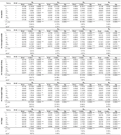
Sensitivity Examination Result
This study analysis model of inducing forward looking information based on the quintile of PB ratio. Model 5 and 6 are analyzed while model 7 did not because model 7 contains collinearity between the change in expected earnings (ΔExit) and the change in
expected growth opportunities (ΔEgit). The
sample is arranged in five partitions and the result is presented in Table 7 as follows.
Table 7 –panel A– exhibits inducing the change in expected earnings based on PB quintile. It indicates that hypothesis HA2 which
stated that the change in expected earnings associates positively with return is supported. This is shown in high level PB for all return types with significance level of 1%, except for Ri1 return type whose significance level of 5%.
It is also shown in medium PB level for Ri1
and Ri4 return types with significance level of,
consecutively, 5% and 10%. Meanwhile, HA1,
HA3, and HA4 are supported consistently as
basic examination previously. Panel B displays inducing the change in growth opportunities based PB quintile. The result indicates that hypothesis HA5 which stated that
the change in expected growth opportunities associates positively with return is supported. It is shown in high PB level with significance level of 1% for all return types. For return type of Ri1 with medium PB level is also supported
with significance level of 10%. Hypotheses HA1, HA3, and HA4, are once again supported
J
o
urna
l of
Indo
nesi
a
n
Eco
n
omy and Business
Ma
y
2
The Result of Inducing the Change in Expected Growth Opportunities Analysis
Notes: Number of observation (N): 6,132. Rit: stock return for firm i during period 1 (1 year), 2 (1 year 3 months), 3 (1 year 6 months), and 4 (1 year 9
months); xit: earnings for firm i during period t; Δbit: change in book value for firm i during period t; Δgit: change in growth opportunities for firm i
during period t; ΔEgit: change in expected growth opportunities for firm i during period t; Δrit: change in discount rate during period t; Δqit: change in
25
3
Coeff. t-value Coeff. t-value Coeff. t-value Coeff. t-value
α ? 0.8341 50.1147 0.0000 *** 0.5030 39.9570 0.0000 *** 0.1857 18.5827 0.0000 *** 0.0403 4.6252 0.0000 *** Xit + 0.1813 8.3607 0.0000 *** 0.0791 4.8235 0.0000 *** 0.0417 3.2009 0.0014 *** 0.0541 4.7685 0.0000 ***
ΔEXit + -0.5064 -2.3509 0.0188 -1.2226 -7.5038 0.0000 -0.6460 -4.9942 0.0000 0.0380 0.3367 0.7363
Δqit + 0.0007 0.0734 0.9415 0.0066 0.9841 0.3251 0.0083 1.5578 0.1193 0.0023 0.4991 0.6177
Δbit + 0.0415 4.4285 0.0000 *** 0.0261 3.6767 0.0002 *** 0.0175 3.1065 0.0019 *** 0.0240 4.8829 0.0000 ***
Δgit + 0.1003 8.9787 0.0000 *** 0.0588 6.9622 0.0000 *** 0.0374 5.5761 0.0000 *** 0.0348 5.9543 0.0000 ***
ΔEgit + 0.0401 8.7008 0.0000 *** 0.0277 7.9435 0.0000 *** 0.0227 8.1983 0.0000 *** 0.0168 6.9515 0.0000 ***
Δrit - 0.0274 2.9270 0.0034 0.0114 1.6089 0.1077 -0.0046 -0.8122 0.4167 -0.0029 -0.6015 0.5476
36.5067 0.0000 *** 22.8584 0.0000 *** 14.9376 0.0000 *** 15.7273 0.0000 ***
4.01% 2.55% 1.68% 1.77%
3.90% 2.43% 1.57% 1.65%
Sig.
F-value
Ri3
Sig. Sig.
Ri4 Pred.
R2 Adj-R2
Ri2
Sig.
Var (s).
Ri1
Notes: Number of observation (N): 6,132. Rit: stock return for firm i during period 1 (1 year), 2 (1 year 3 months), 3 (1 year 6 months), and 4 (1 year 9
months); xit: earnings for firm i during period t; ΔExit: change in expected earnings for firm i during period t; Δbit: change in book value for firm i
during period t; Δgit: change in growth opportunities for firm i during period t; ΔEgit: change in expected growth opportunities for firm i during
period t; Δrit: change in discount rate during period t; Δqit: change in earnings power for firm i during period t is not used to examine hypothesis but
included into model as in basic model. Correlation examination shows that the change in expected earnings (ΔExit) and change in expected growth
opportunities (ΔEgit)have perfect correlation of 0,731, and significant at level 1%. Thus, correlation between both variables is confirmed. ***
Table 7
Sensitivity Examination Based on PB
Panel A:
Inducing
the Change in Expected Earnings
Table 7
Sensitivity Examination Based on PB,
… cont.
Panel B:
Inducing
the Change in Expected Growth Opportunities
Koef. t-value Koef. t-value Koef. t-value Koef. t-value
α ? 0.9288 26.4450 0.0000 *** 0.8136 25.6220 0.0000 *** 0.4895 18.7027 0.0000 *** 0.2148 9.5078 0.0000 *** Xit + 3.6556 15.1250 0.0000 *** 0.7470 3.4187 0.0006 *** 0.4604 2.5564 0.0107 ** 0.6360 4.0915 0.0000 *** Δqit + 0.0581 1.5083 0.1317 -0.0213 -0.6129 0.5401 -0.0172 -0.5992 0.5492 0.0018 0.0747 0.9405 Δbit + 0.0406 2.6430 0.0083 *** 0.0297 2.1406 0.0325 ** 0.0178 1.5593 0.1192 0.0137 1.3860 0.1660 Δgit + -0.7981 -10.5029 0.0000 -0.0549 -0.7993 0.4242 -0.0098 -0.1733 0.8625 -0.0987 -2.0189 0.0437 ΔEgit + -0.1210 -1.4850 0.1378 -0.3143 -4.2688 0.0000 -0.1808 -2.9783 0.0030 0.0365 0.6968 0.4860 Δrit - -1.9144 -9.1785 0.0000 *** -1.3139 -6.9679 0.0000 *** -0.9286 -5.9742 0.0000 *** -0.5916 -4.4101 0.0000 ***
56.8994 0.0000 *** 14.6236 0.0000 *** 10.3056 0.0000 *** 7.6729 0.0000 ***
21.86% 6.71% 4.82% 3.64%
21.48% 6.25% 4.36% 3.16%
Koef. t-value Koef. t-value Koef. t-value Koef. t-value
α ? 0.9222 25.9464 0.0000 *** 0.4938 19.3931 0.0000 *** 0.2327 11.3680 0.0000 *** 0.0867 4.6309 0.0000 *** Xit + 0.1593 1.9848 0.0474 ** 0.1576 2.7409 0.0062 *** 0.1249 2.7013 0.0070 *** 0.2211 5.2293 0.0000 *** Δqit + -0.0085 -0.4580 0.6470 -0.0150 -1.1252 0.2607 -0.0054 -0.5034 0.6148 -0.0153 -1.5653 0.1178 Δbit + 0.0660 1.1642 0.2446 0.0929 2.2854 0.0225 ** 0.0862 2.6384 0.0084 *** 0.1543 5.1654 0.0000 *** Δgit + 0.6958 8.3643 0.0000 *** 0.4835 8.1117 0.0000 *** 0.2673 5.5781 0.0000 *** 0.2123 4.8459 0.0000 *** ΔEgit + 0.0118 0.4103 0.6817 -0.0496 -2.4095 0.0161 -0.0367 -2.2200 0.0266 -0.0108 -0.7140 0.4754 Δrit - -0.0483 -0.7704 0.4412 -0.0552 -1.2301 0.2189 -0.0992 -2.7477 0.0061 *** -0.0683 -2.0676 0.0389 **
13.5731 0.0000 *** 14.9010 0.0000 *** 10.0518 0.0000 *** 11.3842 0.0000 ***
6.26% 6.83% 4.71% 5.31%
5.80% 6.37% 4.25% 4.84%
Koef. t-value Koef. t-value Koef. t-value Koef. t-value
α ? 0.4792 15.5478 0.0000 *** 0.1845 8.5798 0.0000 *** -0.0212 -1.3012 0.1934 -0.0767 -5.0355 0.0000 *** Xit + 1.2576 12.8114 0.0000 *** 0.5891 8.5991 0.0000 *** 0.3452 6.6612 0.0000 *** 0.3829 7.8929 0.0000 *** Δqit + -0.2033 -3.4775 0.0005 -0.0032 -0.0772 0.9385 -0.0011 -0.0365 0.9709 -0.0362 -1.2520 0.2108 Δbit + -0.0251 -1.2186 0.2232 -0.0204 -1.4169 0.1568 0.0060 0.5511 0.5816 0.0231 2.2694 0.0234 ** Δgit + 0.9236 10.5691 0.0000 *** 0.7009 11.4937 0.0000 *** 0.3901 8.4557 0.0000 *** 0.3757 8.7000 0.0000 *** ΔEgit + 0.0179 1.7089 0.0877 * -0.0049 -0.6760 0.4991 -0.0058 -1.0513 0.2933 0.0011 0.2185 0.8271 Δrit - 0.0097 0.3322 0.7398 -0.0114 -0.5553 0.5788 -0.0414 -2.6739 0.0076 *** -0.0382 -2.6355 0.0085 ***
47.2917 0.0000 *** 38.7246 0.0000 *** 23.4348 0.0000 *** 25.7290 0.0000 ***
18.87% 16.00% 10.33% 11.23%
18.47% 15.58% 9.89% 10.80%
Koef. t-value Koef. t-value Koef. t-value Koef. t-value
α ? 0.2745 11.4380 0.0000 *** 0.0812 4.7652 0.0000 *** -0.1054 -7.9728 0.0000 *** -0.1314 -9.9718 0.0000 *** Xit + 1.6042 20.6794 0.0000 *** 0.8755 15.9031 0.0000 *** 0.4960 11.6013 0.0000 *** 0.3664 8.5991 0.0000 *** Δqit + 0.0453 2.4258 0.0154 ** 0.0328 2.4731 0.0135 ** 0.0223 2.1670 0.0304 ** 0.0177 1.7283 0.0842 * Δbit + 0.0260 1.9963 0.0461 ** 0.0130 1.3991 0.1620 -0.0054 -0.7447 0.4566 0.0039 0.5505 0.5821 Δgit + 0.2616 5.1810 0.0000 *** 0.0911 2.5416 0.0112 ** -0.0160 -0.5757 0.5649 0.0218 0.7859 0.4321 ΔEgit + 0.0069 0.6906 0.4900 -0.0057 -0.7953 0.4266 0.0020 0.3569 0.7212 0.0006 0.1125 0.9104 Δrit - 0.0311 2.0845 0.0373 -0.0084 -0.7935 0.4277 -0.0315 -3.8341 0.0001 *** -0.0191 -2.3372 0.0196 **
128.5688 0.0000 *** 71.0870 0.0000 *** 35.4714 0.0000 *** 20.3883 0.0000 ***
38.76% 25.92% 14.86% 9.12%
38.45% 25.56% 14.45% 8.67%
Koef. t-value Koef. t-value Koef. t-value Koef. t-value
α ? 0.4597 22.7135 0.0000 *** 0.1632 11.0796 0.0000 *** -0.1143 -11.1642 0.0000 *** -0.1645 -16.7197 0.0000 *** Xit + 0.1268 4.5959 0.0000 *** 0.0529 2.6357 0.0085 *** 0.0445 3.1890 0.0015 *** 0.0534 3.9825 0.0001 *** Δqit + -0.0011 -0.1140 0.9092 0.0083 1.1756 0.2400 0.0009 0.1928 0.8472 -0.0081 -1.7186 0.0859 Δbit + 0.0140 0.8734 0.3826 0.0049 0.4229 0.6724 0.0078 0.9665 0.3340 0.0148 1.8933 0.0586 * Δgit + 0.0583 5.7255 0.0000 *** 0.0402 5.4251 0.0000 *** 0.0236 4.5824 0.0000 *** 0.0235 4.7377 0.0000 *** ΔEgit + 0.0223 5.6813 0.0000 *** 0.0166 5.8165 0.0000 *** 0.0133 6.7103 0.0000 *** 0.0106 5.5738 0.0000 *** Δrit - 0.0150 1.9462 0.0519 0.0048 0.8491 0.3960 -0.0063 -1.6140 0.1068 -0.0026 -0.6815 0.4957
21.3686 0.0000 *** 13.3140 0.0000 *** 11.6276 0.0000 *** 11.9094 0.0000 ***
9.52% 6.15% 5.41% 5.54%
9.07% 5.69% 4.95% 5.07%
F-value
Sig. Sig. Sig. Sig.
PB
Sig. Sig. Sig. Sig.
Ri2 Ri3 Ri4
Sig. Sig. Sig. Sig.
P
Sig. Sig. Sig. Sig.
Ri2 Ri3 Ri4
Sig. Sig. Sig. Sig.
P
B
R
endah
Var (s). Pred. Ri1 Ri2 Ri3 Ri4
Additional Notes: Number of observation (N) for Low PB: 1,227, Low-Medium PB: 1,226, Medium PB: 1,227, Medium-High PB: 1,226, Medium-High PB: 1,226. The limits for each PB are: Low PB < 0.3065; Low-Medium PB < 0.5462; Medium PB < 0.8505; Medium-High PB < 1.3687, High PB > 1.3687.
Examination using sample partitioning based on PB level shows that hypothesis HA6
which states that discount rate associates negatively with stock price is supported, either
parti-tioning show increase of R2 around 5%-25% and adj-R2 around 4%-24%. Therefore, this sensitivity model has better predictive power than previous models.
Robustness Examination
All examination results of model 5-6 which uses return are re-examined using abnormal return. This examination is aimed to identify the robustness of association for all confirmed variables and investigates its accordance with theory for unconfirmed variables. This examination does not only anticipate systematic risks but also idiosyn-cratic risks. The calculation of abnormal return is based on concept of Fama and French (1992; 1993 and 1995). The regression for all return types indicates that ln(MEit) associates
negatively with return types of Ri1, Ri2, and Ri3
with significance level of 1%, and not signi-ficant for Ri4 return type. Meanwhile,
ln[(BE/ME)it] associates negatively with all
types of return with significance level of 1%. The adj-R2 value for Ri1 is 13.3%; Ri2 is
16,6%; Ri3 is 16,1%; and Ri4 is 8,9%. The
model of Fama and French complete result is presented in Table 8 as follows.
The residuals from four regressions above serve as abnormal return. Then this abnormal return serves as dependent variable to examine additional predictive power. The complete result of robustness examination is presented on Table 9 as follows. The result of model 5 – panel A– which induces the change in expected earnings confirms all hypotheses. All hypotheses HA1, HA2, HA3, HA4, HA5, and HA6
are supported at significance level of 1% or 5% for all Ri1-Ri4 return types. Panel B which
induces the change in expected growth opportunities shows the same result. All hypotheses HA1, HA2, HA3, HA4, HA5, and HA6
are supported with significance level of 1% for all Ri1-Ri4 return types. This robustness
examination shows the highest degree of association for Ri1 return type with R2 as mush
as 5.16% and adj-R2 as much as 5.05% for Ri1
return type. Other return types show lower figures.
Discussion
All examinations show that association and its direction between accounting funda-mentals and stock price movements as hypothesized are supported. This section describes each variables interpretation and concludes in research finding.
Earnings yields and Change in
Expected Earnings Earnings yield and
change in expected earnings associate positively with firm market value. This study supports classical concept (Ohlson, 1995), along with its derivatives studies Lo and Lys (2000), Francis and Schipper (1999), Meyers (1999), Bradshaw, Richardson and Sloan (2006), Cohen and Lys (2006), Bradshaw and Sloan (2002), Bhattacharya, et al. (2003), Collins, Maydew and Weiss (1997), Givoly and Hayn (2000), Kolev, Marquadt and McVay (2008), and Weiss, Naik and Tsai (2008). Eventhough Ohlson (1995) has some weakness that earnings are disturbance when measuring firm market price, this study concludes that earnings is still as a related-cash flow factor of firm value. Therefore, this study indicates that earnings are indicator of value added within accounting matters, and are absolutely reflected in market value.
25
7
Notes: Number of observation (N): 6,132. ARit: abnormal stock return for firm i during period 1 (1 year), 2 (1 year 3 months), 3 (1 year 6 months), and 4 (1
year 9 months); ME
it
: equity for firm i during period t which is calculated by number of outstanding shares multiplied by stock market price; (BE/ME)it
J
o
urna
l of
Indo
nesi
a
n
Eco
n
omy and Business
Ma
y
8
Table 9
Robustness Examination Result
Panel A:
Inducing the Change in Expected Earnings
Coeff. t-value Coeff. t-value Coeff. t-value Coeff. t-value
α ? -0.0813 -5.3704 0.0000 *** -0.0103 -0.9170 0.3592 -0.0170 -1.9002 0.0575 * -0.0370 -4.5447 0.0000 *** Xit + 0.1733 8.7916 0.0000 *** 0.0835 5.7051 0.0000 *** 0.0524 4.4978 0.0000 *** 0.0629 5.9396 0.0000 ***
ΔEXit + 0.5529 2.9111 0.0036 *** -0.4573 -3.2416 0.0012 -0.1134 -1.0102 0.3125 0.3495 3.4232 0.0006 ***
Δqit + -0.0024 -0.2963 0.7670 0.0038 0.6132 0.5397 0.0057 1.1584 0.2467 0.0004 0.0944 0.9248
Δbit + 0.0415 4.7764 0.0000 *** 0.0253 3.9298 0.0001 *** 0.0169 3.2837 0.0010 *** 0.0238 5.0938 0.0000 ***
Δgit + 0.1007 10.0205 0.0000 *** 0.0647 8.6703 0.0000 *** 0.0439 7.3928 0.0000 *** 0.0385 7.1182 0.0000 ***
Δrit - -0.0197 -2.2929 0.0219 ** -0.0272 -4.2519 0.0000 *** -0.0285 -5.5933 0.0000 *** -0.0125 -2.7017 0.0069 ***
52.7621 0.0000 *** 34.4951 0.0000 *** 26.4094 0.0000 *** 25.5695 0.0000 ***
4.91% 3.27% 2.52% 2.44%
4.82% 3.17% 2.43% 2.35%
Pred. ARi1
Sig.
F-value R2 Adj-R2
ARi4
Sig.
ARi3
Sig.
ARi2
Sig.
Var (s).
Panel B: Inducing the Change in Expected Growth opportunities
Coeff. t-value Coeff. t-value Coeff. t-value Coeff. t-value
α ? -0.0548 -4.5167 0.0000 *** -0.0320 -3.5424 0.0004 *** -0.0224 -3.1141 0.0019 *** -0.0203 -3.1102 0.0019 *** Xit + 0.1919 9.5976 0.0000 *** 0.0845 5.6809 0.0000 *** 0.0533 4.5044 0.0000 *** 0.0677 6.2919 0.0000 ***
Δqit + -0.0025 -0.3011 0.7634 0.0042 0.6851 0.4933 0.0058 1.1844 0.2363 0.0002 0.0497 0.9604
Δbit + 0.0400 4.6138 0.0000 *** 0.0247 3.8245 0.0001 *** 0.0166 3.2360 0.0012 *** 0.0236 5.0583 0.0000 ***
Δgit + 0.1118 10.8289 0.0000 *** 0.0668 8.6996 0.0000 *** 0.0449 7.3462 0.0000 *** 0.0407 7.3158 0.0000 ***
ΔEgit + 0.0197 4.8518 0.0000 *** 0.0026 0.8663 0.3863 0.0014 0.5794 0.5624 0.0044 2.0277 0.0426 **
Δrit - -0.0237 -2.7365 0.0062 *** -0.0290 -4.5060 0.0000 *** -0.0291 -5.6845 0.0000 *** -0.0128 -2.7533 0.0059 ***
55.3992 0.0000 *** 32.8168 0.0000 *** 26.2924 0.0000 *** 24.2725 0.0000 ***
5.15% 3.11% 2.51% 2.32%
5.05% 3.02% 2.42% 2.23%
ARi2
Sig.
Var (s). Pred. ARi1
Sig.
ARi4
Sig.
ARi3
Sig.
F-value R2 Adj-R2
Notes: Number of observation (N): 6,132. ARit: abnormal stock return for firm i during period t, 1 (1 year), 2 (1 year 3 months), 3 (1 year 6 months), and 4 (1
year 9 months); xit: earnings for firm i during period t; ΔExit: change in expected earnings for firm i during period t; Δbit: change in book value for firm
i during period t; Δgit: change in growth opportunities for firm i during period t; ΔEgit: change in expected growth opportunities for firm i during period
t; Δrit: change in discount rate during period t; Δqit: change in earnings power for firm i during period t is not used to examine hypothesis but included