Kollektiivisen liikkeen ohjaaminen

(1)

Aalto University School of Science

Degree Programme of Engineering Physics and Mathematics

Markus Karppinen

Steering collective motion

Master’s Thesis

Espoo, January 18, 2013

Supervisor: Professor Jouko Lampinen Instructor: Professor Jari Saramäki

(2)

Aalto University School of Science

Degree Programme of Engineering Physics and Mathematics

ABSTRACT OF MASTER’S THESIS Author: Markus Karppinen

Title:

Steering collective motion

Date: January 18, 2013 Pages: 54

Professorship: Computational Science Code: BECS-114 Supervisor: Professor Jouko Lampinen

Instructor: Professor Jari Saramäki

Collective motion is an umbrella term for both biological and non-organic coherent motion, in which tens to tens of millions units take part in. The huge fish schools that fishing ships pursue and the nightmarish legions of locusts which destroy entire countries’ worth of crops are just a few examples of collective motion in nature that have a direct effect on us humans.

This thesis focuses on the complex behavior of collective motion and studies how such movement can be steered. As a tool, the original Vicsek model for simulating collective behavior is used. An agent-based model, the Vicsek model was introduced in 1995 and has been extensively utilized and studied since. The Vicsek model consists of units that move independently but prefer to take the common movement direction of their neighbors. Although it is a simplified model, the Vicsek model exhibits flocking behavior that is similar to what is observed in nature.

The results of this thesis show that in this context, collective motion of hundreds of units is greatly affected by just a small percentage of special units, called leaders. The leaders don’t adhere to the common rules of the other units, but move in a constant direction. It is observed that the relative amount of leaders needed to steer the entire flock actually decreases as the flock size grows or if we wait sufficiently long. This leads to the conclusion that in the limit of an infinite system size, a finite amount of leaders would suffice to control the flock.

Keywords: collective motion, flocking, swarming, locusts, agent-based modeling, Vicsek Model, leader units

Language: English

(3)

Aalto-yliopisto

Perustieteiden korkeakoulu

Teknillisen fysiikan ja matematiikan tutkinto-ohjelma

DIPLOMITYÖN TIIVISTELMÄ Tekijä: Markus Karppinen

Työn nimi:

Kollektiivisen liikkeen ohjaaminen

Päiväys: 8.1.2013 Sivumäärä: 54

Professuuri: Laskennallinen tiede Koodi: BECS-114 Valvoja: Professori Jouko Lampinen

Ohjaaja: Professori Jari Saramäki

Kollektiivinen liike on kattotermi sekä biologiselle että ei-orgaaniselle koherentil-le liikkeelkoherentil-le, johon osallistuu kymmenistä kymmeniin miljooniin yksikköä. Luon-nossa esiintyvä kollektiivinen liike vaikuttaa suoraan meihin ihmisiinkin, kuten esimerkiksi kalastuslaivastojen metsästämät kalaparvet tai valtavat kulkusirkka-parvet jotka tuhoavat kokonaisten valtioiden viljasatoja osoittavat.

Tämä diplomityö keskittyy kollektiivisen liikkeen kompleksiseen käytökseen sekä tutkii kuinka tällaista liikettä voidaan ohjata. Työkaluna käytetään kollektiivisen käytöksen simuloimiseen tarkoitettua Vicsekin alkuperäismallia. Vicsekin malli on agenttipohjainen malli joka esiteltiin vuonna 1995, ja jota on siitä lähtien käy-tetty ja tutkittu laajasti. Vicsekin malli koostuu yksiköistä jotka liikkuvat itsenäi-sesti, mutta suosivat läheisten yksiköiden keskimääräistä liikesuuntaa. Vaikkakin Vicsekin malli on yksinkertaistettu, sen tuottama parvikäytös vastaa luonnossa havaittavaa käytöstä.

Tämän diplomityön tulokset osoittavat satojen yksikköjen kollektiivisen liikkeen käytöksen olevan riippuvainen vain pienen prosenttiosuuden muodostavien eri-tyisten johtoyksiköiden käytöksestä. Johtoyksiköt eivät noudata samoja sääntöjä kuin muut yksiköt, vaan liikkuvat vakiosuuntaan. Kun parven koko kasvaa tai odotettaessa riittävän kauan, koko parvea ohjaamaan tarvittavien johtoyksiköi-den suhteellinen lukumäärää vähenee. Tästä voidaan päätellä että äärettömän kokoisessa systeemissä äärellinen määrä johtoyksiköitä riittää kontrolloimaan ko-ko parvea.

Asiasanat: kollektiivinen liike, parveilu, kulkusirkka, agenttipohjainen mallintaminen, Vicsekin malli, johtoyksikkö

Kieli: Englanti

(4)

Preface

This work was carried out at Aalto University School of Science, the Depart-ment of Biomedical Engineering and Computational Science.

This is as good a time as any to officially thank those who have especially helped in making this thesis a reality, like Paavo Niskala who let me use his code as a foundation for my own; Jelena Luketina who read and commented on the thesis in a crucial phase; Joonas Piili and Ville Backlund, the guys in my room, for advice and company; Lauri Kovanen and Mikko Kivelä for being older and wiser than me but still willing to offer invaluable advice; and of course the rest of the research group.

The biggest thank you, however, goes to a supervisor who has gone above and beyond any duty he might have had and instead mentored, helped and guided me for years. Jari, without your input I would never have made it this far!

Otaniemi, Espoo, January 18, 2013

Markus Karppinen

(5)

Symbols

N total number of units NL number of leaders

φ average normalized velocity

η noise

− →_v

i the velocity of particle i

− →_x

i the position of particle i

ϑi(t) the angle of the direction of motion at time t

R interaction range

θi the angle of motion of theith particle

ηA the amplitude of noise

ξ uniformly distributedδ-correlated white noise A adjacency matrix

aij element in ith row and jth column in the adjacency matrix

β tuning parameter affecting the strength of influence L side length of simulation area

ρ unit density

pL probability that the flock is following the leader

Abbreviations

SPP self-propelled particle VM Vicsek Model

ABM agent-based model/modeling AN angular noise VN vectorial noise BU backward update FU forward update CSM Cucker-Smale model 5

(6)

List of Tables

2.1 The different variants of the Vicsek model considered . . . 31

4.1 The parameters used for the flock simulations. . . 40

4.2 The parameters used for critical simulations. . . 46

4.3 The critical values from the size and time simulations. . . 47

(9)

List of Figures

1.1 A flock of starlings demonstrating the shape-shifting capabilities of flocks. Source: www.flowingdata.com . . . 12 1.2 Overhead snapshot of robotic koi predator with live

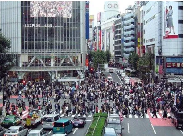
golden shiner school in a tank [6]. . . 15 2.1 People crossing the street in the crowded Shibuya,

Tokyo, Japan. Source: http://blogs.usyd.edu.au/theoryandpractice/ 2006/10/japan_travelgoue.html . . . 17 2.2 The behavior of the order parameter φ ∈ [0,1] as a

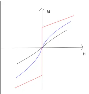
function of system noise η. The left side represents a first-order phase transition, defined by the non-continuous behav-ior exhibited. The right side represents a second-order phase transition, and is smooth. . . 20 2.3 The behavior of magnetization M in an external field

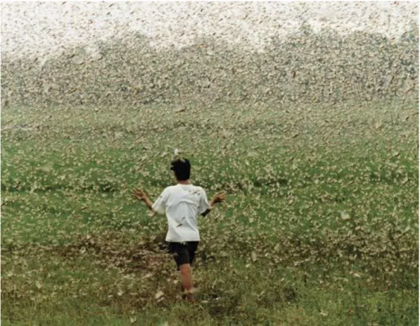
H, an example of system size affecting the behavior of the system. The gray line is a small-sized system, the blue one is a large-sized system, and the red one is an infinite-sized system. The bigger the system, the more ideal the transition. 21 2.4 A farmer caught in a huge locust swarm. Source: http:

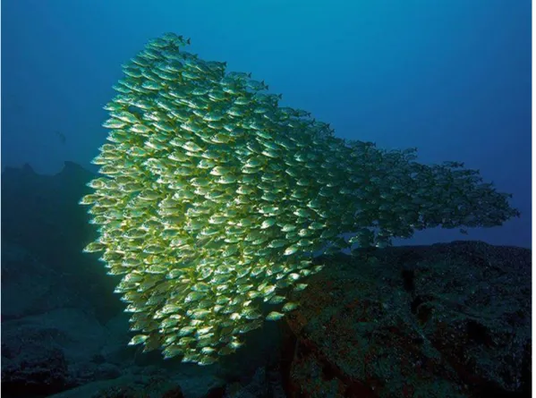
//knowingthese.blogspot.fi/2010/06/insect-swarms-problem. html . . . 24 2.5 A close-swimming fish school can manage

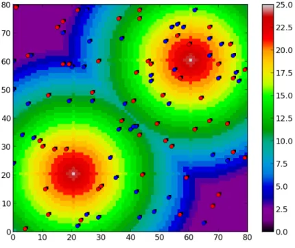
lightning-quick movements without the fish bumping into either other fish or obstacles. Source: http://caesarom.com/ . . . 25 2.6 A picture of the Sugarscape, as an example of an

ABM.The red and blue dots are units that scavenge for food (indicated by the background color of the lattice), and try to survive. [19] . . . 28

(10)

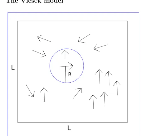
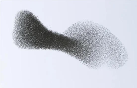
2.7 Illustration of the Vicsek model. The arrows are "birds", units that fly in the direction of the arrow with a constant velocity. The blue circle shows the interaction range R, i.e. the bird takes the average direction of the birds within a circle around it. The area where the system is simulated is a square with side length L with periodic boundary conditions. . . 30 2.8 A picture from a study of marching locusts. The

lo-custs circle around the container, until suddenly they simulta-neously change directions. This has been explained by the accumulation of small errors made by the locusts as they try to mimic the motion of their neighbors. Source: http: //www.kurzweilai.net/social-networking-for-locusts . . . . 36 4.1 The order parameter as a function of system noise.

Each data point is an ensemble average of 50 runs made. The valueη = 0.5 is chosen as it is clearly in the non-zero area. . 41 4.2 An example of how leaders affect the behavior of the

flock, with NL = 10. The leaders are marked and circled in

red. As time passes, the birds form flocks which merge into bigger flocks. The leaders take control of the flocks and most birds fly in the direction φ= 0 (with some perturbations due to noise). The black circle shows the range of interaction. . . 42 4.3 Four examples of the flock’s average flight direction as

a function of time, with flock size N being 500. The red line indicates the leaders’ flight direction. The closer the dots are to the red line, the more the units are flying in the same direction as the leaders. . . 44 4.4 The probabilitypLthat the flock is following the leader

at the end of 200 cycles as a function of the amount of leaders. N = 500, L = 25 and ρ = 0.8. Each data point is an average of 100 runs. . . 45 4.5 The effect of system size on the leader’s and their flock

"hijacking". . . 46 4.6 The effect of waiting time window choice on the

"hi-jacking" of the flock. If every value of the order parame-ter in the time window is between [−₈π,π₈], then the flock has adopted the leader’s flight direction. . . 47

(11)

11

4.7 The effect of system size and waiting time on the "hi-jacking" of the flock. Clearly the bigger the system and the longer we wait, the less percentage of leaders is needed to steer the entire flock into the direction wanted. The lower pictures show the inverse of both system size and waiting time. By making an approximate fit to the part closest to zero, we can extrapolate to find the probable point where the curve intersects the y-axis. This corresponds to the ideal limit N(τ) → ∞,_N1(1_τ)→ 0. In reality the value for both is about

0.2%. . . 48 5.1 An army of ants demonstrating the power of

coopera-tion. Source: http://fofoa.blogspot.fi/2010_04_01_archive. html . . . 51

(12)

Chapter 1 Introduction

Figure 1.1: A flock of starlings demonstrating the shape-shifting capabilities of flocks. Source: www.flowingdata.com

Living in a world with crowded cities, coral reefs full of fish schools and skies filled with both insect swarms and bird flocks, synchronized movement surrounds us in all directions. A huge number of units moving in unison, ducking and rolling across skies or ocean floors, is one of nature’s magnifi-cent displays of physics in action. Collective motion can be at the simplest defined as just synchronized movement of many units of the same type. A sub-field of collective behavior, collective motion is, however, a lot more

(13)

CHAPTER 1. INTRODUCTION 13

verse than can be expected at first glance. The science of collective motion builds on experimental results in the wild, but also on results from physics and computer simulations. Uniting biology, physics and computer science, it is a try to create an understanding of what makes flocks tick.

What makes flocks, schools and swarms so interesting is the great speed and agility of the group as a whole, i.e. the ability of the group to behave as a single entity while consisting of a great number of simple biological units. Without bumping into each other or into obstacles, the units can achieve great coordination and a flock behaves almost like a fluid. This behavior is characteristic of swarms which are so large that information can’t possibly travel from one side of the flock to the other fast enough so that all units could be aware of the actions of all other units. This has led some experts in the past to cite even telepathy as a means of communication in a swarm. However, it has turned out that such behavior can arise from fairly simple rules of interaction between the members of a swarm. Such rules of interac-tion are readily investigated with computer simulainterac-tions of swarming behavior. The forerunner in studying flocking behavior using simulation, C.W. Reynolds, pretty much initiated the field in 1987 with his seminal paper [1]. The next leap forward was the Vicsek model [2] in 1995, where statistical physics was fused with algorithmic treatment of flocks. Since our focus is in steering collective motion, a crucial paper that came out in 2000 is [3], where an actual experiment shows that a flock consisting of golden shiners, a type of small fish, can be hijacked and steered to a location of the experimenter’s choosing using trained individuals. There have been some books on collective motion, e.g. [4] which focuses on designing and optimizing complex systems based on models of social insect behavior. I also reference throughout this thesis Vicsek’s detailed review paper on collective motion [5], which came out in early 2012, and is pretty much the latest word on this rich field of study.

This thesis focuses on mathematical modeling of collective motion, and computer simulations of swarming behavior. In particular, I aim to study how one can affect collective motion, and how difficult it is to steer a herd or a school in the desired direction by manipulating the behavior of a small number of its units. This setting is inspired by recent empirical results, where actual fish schools were manipulated by inserting robot fish, who could then guide the rest of the school to a desired position in the fish tank [6]. Figure 1.2 is taken from the same paper, and it shows a robotic predator in a tank with a real fish school.

(14)

As a tool I use a simple toy model, the Vicsek Model (VM), which has been studied comprehensively [5] since its inception in 1995. VM is an agent-based model, where many units depicting fish or birds interact with all other units within a certain interaction range. They correct their flight direction to match the neighboring units, and thus form flocks that move coherently.

In addition to a better understanding of insect swarms and fish schools in nature, I am motivated by the possibility of man-made, robotic swarms and their control. The robot revolution has been coming for a long time, and it might not be long before simple helper robots are as common-place as cell phones today. Before this can happen though, we will need to be able to program the robots to abide by the subconscious social norms which govern our movement through the thick that is rush hour pedestrian traffic. Additionally, in settings such as disaster relief swarms of robots may prove to be very useful e.g. in locating earthquake victims or inspecting damaged in-stallations deemed too dangerous for humans. Unless technological advances enable such swarms to operate autonomously, they need external guidance and direction, which of course is slow, cumbersome and expensive.

What I intend to do is to study how one can control collective movement. Is it possible to take a toy model of swarming behavior and modify it so that the flock flies in the direction one wants, if only a small fraction of the swarm members obey some directional preference? How big a percentage has to be controlled before we can steer the swarm? Would it be possible to further extend this into the real world and e.g. take control of huge locust swarms and direct their movement away from inhabited areas and so spare the crops of many a poor farmer or to help fish without causing widespread environ-mental damage in the process? These are questions with large stakes, and I’ll try to answer the first two, while leaving the last ones for robot engineers and biologists.

(15)

Figure 1.2: Overhead snapshot of robotic koi predator with live golden shiner school in a tank [6].

(16)

Chapter 2 Theory

2.1 Collective motion - basics

Collective motion is a part of a greater class of phenomena called collective behavior, of which there is a huge variety of systems stretching over many orders of magnitude. Collective behavior can be defined as action where the system’s units interact with each other locally, which gives rise to emer-gent behavior on a system-wide scale. We assume that a system exhibiting collective motion is made out of units that

(a) are quite similar,

(b) can change their direction of movement, (c) have a specific interaction range and

(d) are subject to varying amounts of noise, i.e. random perturbations in their movement direction [5].

Starlings, for example, form big flocks1 that can consist of hundreds of birds. They can change their direction of flight quickly, but still they stick close to each other so that the flock looks almost as a blob of liquid when viewed from afar (see Figure 1.1). Another example is human rush hour pedestrian traffic. Everyone is moving at pretty much the same pace and no matter how crowded the street, people still manage to not bump into each other too hard (see Figure 2.1). Thus it’s very rare that anyone walks into someone so hard that they would fall down or get injured.

1_{Flocks of starlings are actually called murmurations, as a part of the long tradition of}

many species having their own collective nouns in English.

(17)

CHAPTER 2. THEORY 17

Collective behavior is not limited only to macrobiological systems, how-ever. Although one of the ways to define life is to ask the question: ’does it move on its own accord?’, it has recently been found out that also sev-eral physical and chemical systems possess interacting, "self-propelled" units, or particles, known shortly as SPPs. Collective motion has been observed in non-living systems such as shaken metallic rods, simple robots, boats, etc. in addition to living systems such as macromolecules, bacterial colonies, amoeba, cells, insects, fish, birds and mammals including humans.

Figure 2.1: People crossing the street in the crowded Shibuya, Tokyo, Japan. Source: http://blogs.usyd.edu.au/theoryandpractice/ 2006/10/japan_travelgoue.html

The mechanisms or "rules" of interaction between many similar units, such as molecules, bacteria, flocks of birds or schools of fish, can be very simple as we’ll see, or a complex combination of many simple interactions. These interactions can take place between neighbors in 2D or 3D space, or be mediated through an underlying lattice or network. Also the medium itself can affect the interactions: e.g. in a dissipative medium the interactions may

(18)

have shorter range, and external fields such as wind or magnetic fields can affect the movement of the particles. As with many complex systems, the complexity itself emerges from unit-to-unit interactions.

With collective motion defined, the choice of methodology must be made carefully. Comparing diverse motion patterns, we have to ask ourselves, are these system-specific or general? In biological sciences it is common that all cases differ, with every new case being mostly unique. For example all bird species have their own nesting and mating behavior, which have developed with time. In statistical physics, however, many seemingly unique phenom-ena can be grouped under just a few universality classes. For example, the behavior near a second order phase transition coincides in very different phe-nomena, such as magnetic systems, superfluid transition and alloy physics. As a physicist I opt for the second approach, but in reality the truth probably lies somewhere in between.

There are a lot of good reasons why swarming and flocking is so widely observed in nature, i.e. the benefits greatly outweigh the potential draw-backs of staying closely together. When the units stick together, they are a lot safer when a predator appears than what they would be if they were on their own. Not only are big fish schools, for example, harder to attack with the flock outsizing any marine predator, but if need be the flock can disperse and hence significantly lower the probability of a single unit being caught. Flocking is also beneficial for exploration for resources or hunting, as many units can cover a bigger area and communicate any finds to the rest of the flock. Decision-making is also improved in larger groups, as in many cases practically any unit can initiate a group movement and hence reach the intended goal without scattering or conflicts taking place.

In the previous few decades a lot of information has amassed due to the myriad of experiments and observations done in the field [5]. We now know that movement and a tendency to adopt the direction of motion of the neigh-bors is the main reason for collective ordered motion. It’s been noted that very similar behaviors occur in systems of very different origin and both 2D (land-based) and 3D (aquatic or marine) systems contain many more similar-ities than one would expect. This suggests the possibility of the existence of universal classes of collective motion patterns. Also, boundary conditions sig-nificantly affect the essential features of flocking. Collective decision making is usually made in a globally highly disordered, locally moderately ordered state.

(19)

The simplest forms of collective motion can be found in systems where all members can be considered identical. Many insect, fish and bird species live in big groups, where they may be unable to recognize each other at the level of individuals. In these cases leadership is usually only temporary (e.g. for as long as an informed individual leads the flock to food), or non-existent, i.e. the movement is dictated by a general consensus that is formed by some units moving in a random direction and other units imitating the movement of them. Mammals, on the other hand, have the capacity to recognize in-dividuals, and hence can form hierarchical groups, where certain individuals permanently act as leaders.

It is thus an important question how flocks of animals form the common decision to move in a coherent way. Two different mechanisms have been suggested in the literature [7]: "Consensus decision" is a process in which the members of a group choose between two or more mutually exclusive ac-tions with the aim of reaching a consensus. "Leadership" on the other hand is the initiation of new directions of locomotion by one or more individuals, which are then followed by other group members. As mentioned before, such leadership can be either permanent or temporary, depending on the species and situation.

Generally, collective decision-making can be divided into two rules: ’indi-vidual-based’ and ’self-organized’ [5]. Individual-based consists of differences in social status, physiology, inner state, etc. Self-organization refers to pas-sive interactions and simple, automated responses among individuals.

2.2 The physics of collective motion

In various models of flocking, coherent motion emerges through a transition from an unordered state to an ordered as a function of the parameters of the models. Thus to understand the theory of collective motion we need to know the physics behind such transitions. For example, here has been quite a lot of discussion about whether one of the simplest of models depicting collective motion, the Vicsek model, introduced in [2], has a continuous or discontinu-ous phase transition where the disordered motion of the flock is replaced by unidirectionality. But what exactly is a phase transition and what do such transitions have to do with SPPs?

(20)

consist-CHAPTER 2. THEORY 20

ing of a huge number of interacting particles, undergoes a transition from one phase to another, typically from a disordered into an ordered phase, as a function of one or more external parameters [5]. A typical example of this process is the freezing of water, when a liquid becomes a solid. The degree of order and symmetry of a phase is characterized by the order parameter. Mathematically, this value is usually zero in the disordered phase and non-zero in the ordered phase.

When it comes to collective motion, the parameter usually chosen is the average normalized velocity φ,

φ= 1 N v0 | N X i=1 − →_v i| (2.1)

where N is the total number of the units, v0 is the average absolute

ve-locity of the units in the system and −→v i is the vector of velocity of particle

i.

If the motion is disordered, the velocities of the individual units point in random directions and average out resulting in a velocity vector of small magnitude, whereas for ordered motion the velocities all add up to a vector of absolute velocity close to N v0. Thus the order parameter for large N can

vary from about 0 to about 1.

Figure 2.2: The behavior of the order parameter φ∈[0,1] as a func-tion of system noise η. The left side represents a first-order phase tran-sition, defined by the non-continuous behavior exhibited. The right side represents a second-order phase transition, and is smooth.

There are two kinds of phase transition, first and second order, named so due to the behavior of the derivatives of the parameter. If the order

(21)

param-CHAPTER 2. THEORY 21

Figure 2.3: The behavior of magnetization M in an external field H, an example of system size affecting the behavior of the system. The gray line is a small-sized system, the blue one is a large-sized system, and the red one is an infinite-sized system. The bigger the system, the more ideal the transition.

eter changes discontinuously during the phase transition, the transition is defined as a first-order transition, and it contains a latent amount of energy, e.g. latent heat. Latent heat is the heat released or absorbed by a body or a thermodynamic system during a process that occurs without a change in temperature. Sticking to the example of water, when melting ice the tem-perature does not rise above zero until all the ice has been converted into water. Only then does the energy start going to heating the water.

In second-order transitions, on the other hand, the order parameter changes continuously, while its derivative is discontinuous. Second-order transitions are always accompanied by large fluctuations of some relevant quantities at the transition point. See Fig. 2.2 for a visual example. Phenomena as-sociated with a continuous phase transition are called critical phenomena. This is because the transition takes place at an exact critical point. Near the critical point, the behavior of the quantities describing the system are very sensitive to small perturbations, and are characterized by the so-called critical exponents.

(22)

Ising model [8], we have particles with either spin up or down, with their collective behavior accounting for macroscopic magnetization of a physical body. Depending on the temperature the system has two separate phases; a disordered one where the particles have random spin, and an ordered one where the particles have the same spin, also known as the magnetized phase. At low temperatures the spins of the particles align themselves to imitate the spins of nearby particles, but as temperature rises the couplings of the spins are broken by thermal motion. If we have an external field, the spins align themselves according to the field. System size is a key factor in how the magnetization behaves: the bigger the system, the steeper the transition from one phase to another, as can be seen in Figure 2.3. For finite-size sys-tems, the transition is always somewhat smeared-out, and becomes sharp at the thermodynamic limit of infinite system size.

A key physical element of collective motion is noise (η), the added ran-domness to the direction of motion, caused by the unideal nature of interac-tions. When it comes to systems of SPPs, noise plays the order-destructive role of temperature. The flock behaves less coherently if the units have big-ger uncertainty of the locations and velocities of their neighbors, and will break down if the value of the noise becomes too large. Interestingly, various different physical systems follow similar laws and even their different critical exponents are related to each other. It is worth noting that the results of statistical physics are only exact in the thermodynamic limit, i.e. when the number of particles of the system tends to infinity. Often the number of units participating in collective motion is far from the huge quantities of particles that statistical physics usually deal with. Most real-life observations and experiments involve this mesoscopic scale of a few dozen to a few thousand SPPs.

2.3 Observations and experiments

The main difficulty in observations and experiments concerning collective motion is to keep track of all the trajectories and in some cases velocities of all the particles. This is because there are many particles and they are both almost indistinguishable and moving very fast in unpredictable ways. We have only recently started to understand the rich variety of phenomena that are connected to collective motion and the fact that also non-living particles can participate. Still, there have been many ingenious experiments devised to observe this fascinating phenomenon.

(23)

2.3.1 Inanimate objects

This thesis does not focus on collective motion at the cellular level or in inanimate objects, but it is worth noting that there have been some rele-vant results. In a recent experiment [9], researchers have studied inanimate objects using commercial radio-controlled boats moving in a circular pool, interacting through inelastic collisions only. Using varying amounts of noise in the communication between boats, various kinds of patters were recorded, such as clustering, jamming, disordered and ordered motion, depending on the noise level. It was also found that a few steerable boats, which acted as leaders, were able to "hijack" the group and steer its movements. To do this, it was enough to manipulate just 5 to 10 % of the boats.

When it comes to inanimate objects, such as metallic rods shaken in a container where they form swarm-like clusters, the assumption that only a few parameters and factors dictate the emergence of collective motion is in-creasingly supported [5]. It has turned out that one of these parameters is the particle density, or the density of the objects, inanimate or living, that exhibit collective motion.

2.3.2 Insects

One of the prime examples that comes to mind when mentioning collective motion are ants. They use pheromone trails to create tracks between the nest and food sources and move efficiently between the two. For example, New World army ants stage huge swarm raids with up to 200 000 individuals forming trail systems that are up to 100 meters long and 20 meters wide [5]. However, the chemical signaling used by ants is somewhat a special case, and coordinated movement in insects may be driven by mechanisms as sim-ple as physical collisions. As an examsim-ple, it has been shown that coordi-nated marching behavior in marching locusts strongly depends on the animal-density, and is mostly caused by the locusts’ cannibalistic tendencies. The locusts are actually just trying to eat each other, but the emergent phe-nomenon is a huge swarm moving in a coordinated way. The transition between disordered and ordered states has been shown to exhibit hysteresis and a behavioral first order phase transition [10].

(24)

Figure 2.4: A farmer caught in a huge locust swarm. Source: http: //knowingthese.blogspot.fi/2010/06/insect-swarms-problem.html

2.3.3 Fish

Two terms, "shoal" and "school" are commonly used to describe collective groups of fish. These terms carry different meanings. In a shoal fish relate to each other in a looser manner than in a school, and they might include fish of various species. Shoals are more vulnerable to predator attack, whereas in a school fish swim in a more tightly organized way considering their speed and direction [5].

Fish schools are typically leaderless aggregations of individuals following selfish survival strategies, with only a limited range of observation. Only the few outer layers of the school can actually access external stimuli from out-side the school. The majority of fish relay on social cues from their neighbors for information about the school’s environment. For example, an individual fish that does not perceive a predator directly can react to a neighbor turn-ing fast and compensate its movement to match that of its neighbors, thus

(25)

staying with the school and avoiding the predator [6].

Figure 2.5: A close-swimming fish school can manage lightning-quick movements without the fish bumping into either other fish or ob-stacles. Source: http://caesarom.com/

The trajectories of young fish in a school were studied in [11]. Both indi-vidual and collective behavior were studied as a function of animal density and a transition from disordered to ordered motion was noted. It was exper-imentally shown that fish behave like attracting entities, selecting the mean orientation of their neighbors. The interactions between schooling golden shiners were studied in [12]. It was found that changes in speed are the main form of interaction between the fish, and alignment only modulates the strength of speed regulation, instead of being a force in itself. The forces that do play a role are attraction and repulsion, as could be expected from other results.

Herring populations spanning over tens of thousands of square kilome-ters were observed during spawning using a technique called ’Ocean Acoustic

(26)

Waveguide Remote Sensing" (OAWRS) [13]. A rapid transition from disor-dered to highly synchronized behavior was observed at a critical population density. It was found that a small set of leaders can significantly influence the actions of a much larger group. Pretty much the same conclusion was reached when Reebs et al. [3] trained twelve golden shiners to expect food around midday in one of the brightly lit corners of their tanks. Then the informed individuals were placed in uninformed shoals. It was examined whether the trained individuals could lead their uninformed shoal-mates to the food-site. Surprisingly, as few as a single informed individual was enough to guide the entire shoal to the food. Interestingly, the shoals never split up into smaller parts and they were always led by the same fish.

2.3.4 Birds

When bird movement was studied through a frame-by-frame analysis of high-speed film of sandpiper flocks in [14], it was argued that any individual can initiate a flock movement. When initiated, the movement propagates through the flock in a wave-like form radiating in all directions from the initiation site. Very high propagation speeds are achieved by individuals observing ap-proaching maneuver waves and timing their own execution to coincide with its arrival, just as sports fans doing "the wave" demonstrate.

In the EU FP6 NEST project Starflag [5], the team measured the 3D positions of individual European starlings in flocks containing up to 2600 birds using stereometric and computer vision techniques. They studied the angular orientation of each bird and its nearest neighbors and found that starlings only interact with their 6-7 closest neighbors. This is known as a "topological approach", in contrast to "metrical approach" where the birds interact with others within a given distance. There have been opposite views expressed since, and the interaction mechanism is still unclear, but it is pos-sible that the approach differs from species to species.

Studies on homing birds have shown that when a pair of birds is flying to-gether the actions depend on the amount of difference in preferred direction. With small disagreements most pairs studied averaged out their routes, but upon reaching a critical threshold in disagreement, the pairs either split up or one of the birds became the leader [15]. It was also observed that almost all pairs navigated more efficiently than the individuals they were composed of, even if there was no leadership present.

(27)

2.3.5 Mammals

Leadership in zebras has been divided into effects of identity, i.e. dominance and kinship relations, and inner state, i.e. whether the individual is in its lactation period. As investigated in [16], lactating females initiated group movement more often than non-lactating ones, which points towards inner states having an important role in leadership. Put simply, those individu-als with the greatest motivation to move will most vigorously try to initiate group movements. Beef cows, however, seem to initiate short-distance travel and foraging movements in a graded manner, i.e. the higher an individual is in the group hierarchy, the bigger influence it can have on the movements of the herd [17].

2.3.6 Robots

The first steps towards robots interacting amongst human populace have been taken by building and studying simple robots following a few basic rules: avoidance, aggregation, dispersion and homing. With these rules the scientists were able to achieve flocking behavior. Turgut et al. [18] exam-ined the swarming of units which were equipped with a digital compass, an infrared-based short range sensing system, and other tools for sensing the di-rection of other units. They found that the main factor for defining the size of the swarm is the communication range between units, and that the size is robust against the amount and nature of the noise disturbing the sensing systems and the number of neighbors a unit has.

2.4 Models and simulations

2.4.1 A quick look at agent-based modeling

There are many different models used for studying and simulating collec-tive motion in a variety of dimensions, and the most use an agent-based approach [5]. Agent-based modeling (ABM) is a common term for computer simulation models where the system consists of several autonomous units, agents, that follow simple rules, which lead to system wide complex behavior by way of emergence from the micro level to the macro level. As an example of an ABM, Figure 2.6 (taken from a special assignment done by the author) shows a model called the Sugarscape, where units eat, breed and evolve.

(28)

Figure 2.6: A picture of the Sugarscape, as an example of an ABM. The red and blue dots are units that scavenge for food (indicated by the background color of the lattice), and try to survive. [19]

Using ABM to study collective motion is useful, as it links the simple rules followed by the agents and the emergent behavior of the swarm. Here’s a list of common rules applied in many agent-based models used in studying collective motion [5]:

(i) a long-range force avoiding being alone, e.g. moving towards the center of the swarm’s mass

(ii) short-range repulsive force aiming to avoid collision with flock-mates and obstacles

(iii) adjusting the velocity vector according to the rest of the flock, e.g. taking the direction of the neighboring units

(iv) noise, i.e. random added perturbations to the unit’s movement

(v) some kind of optional drag force caused by the medium in which the individuals move

(29)

There are some limitations in ABMs; different combinations of rules and parameters may provide similar patterns and collective behaviors. Hence, it’s not enough to provide a rule and a parameter set and demonstrate that they reproduce observed behavior. This will not prove that a certain bio-logical system obeys some given principles [20]. On the other hand, it has been demonstrated in [21] that the same rule and parameter set may result in different collective behavior, even in the same system, depending on the history of the system. It was however, noted in the same paper that their model led to the first evidence for collective memory in animal groups, i.e. the previous history of group structure influencing the collective behavior ex-hibited. Using ABMs might be a double-edged sword, but they still remain a useful tool for testing emergent behavior.

2.4.2 Precursors: The Reynolds and Aoki models

The model of Reynolds [1] is one of the first widely-known flocking simula-tions. He studied bird-like particles, called "boids", moving along trajectories defined by differential equations. He took into account only three types of interactions:

(a) Separation: trying to maintain a safe distance in order to avoid crowding or colliding with flock-mates, using the metrical approach.

(b) Alignment: objects steer towards the average heading direction of their local flock-mates and mimic their movements.

(c) Cohesion: objects move towards the average position of their neighboring flock-mates.

The boids of Reynold’s model work independently and try both to stick together and avoid collisions with one another and with objects in their vicin-ity. Boids released near another begin to flock together forming small groups with its members heading approximately in the same direction and they change direction in synchronization. Smaller groups join to become bigger flocks and when they encounter external obstacles the flocks can split into smaller groups. The original simulations also corresponded visually to how flocks look like in nature and gave further confirmation that the model was onto something.

Even earlier, Aoki used pretty similar rules to simulate the collective mo-tion of fish [22]. The units adhered to rules of avoidance, parallel orientamo-tion

(30)

movements and approach.

The speed and direction of the units were stochastic in this model, but the direction of the units was related to the location and heading of the neigh-bors. It was also stated that collective motion can occur without a leader and that the individuals don’t need information regarding the movement of the entire flock.

2.4.3 The Vicsek model

Figure 2.7: Illustration of the Vicsek model. The arrows are "birds", units that fly in the direction of the arrow with a constant velocity. The blue circle shows the interaction range R, i.e. the bird takes the average direction of the birds within a circle around it. The area where the system is simulated is a square with side length Lwith periodic boundary conditions.

A versatile and well-studied toy model, the Vicsek model (VM) [2] takes its approach from statistical physics. This makes it possible to study more quantitatively the behavior of huge flocks in the presence of noise. Another benefit is the model’s simplicity as it only has one rule: at each timestep a

(31)

given particle driven with a constant absolute velocityv0assumes the average

direction of motion of the particles in its neighborhood of radiusRwith some noise/perturbation added. For a concept sketch of the model, see Figure 2.7. The simulations of VM are done in two dimensions where pointlike par-ticles move continuously and without a lattice in an area with a finite side-lengthLwith periodic boundary conditions. Each particle (or unit) is labeled with an integer index (i) and hence its position and velocity are denoted by

− →_x

i and −→v i. As stated above, the absolute value of velocity of all units is

constant, i.e. vi =v0,∀i.

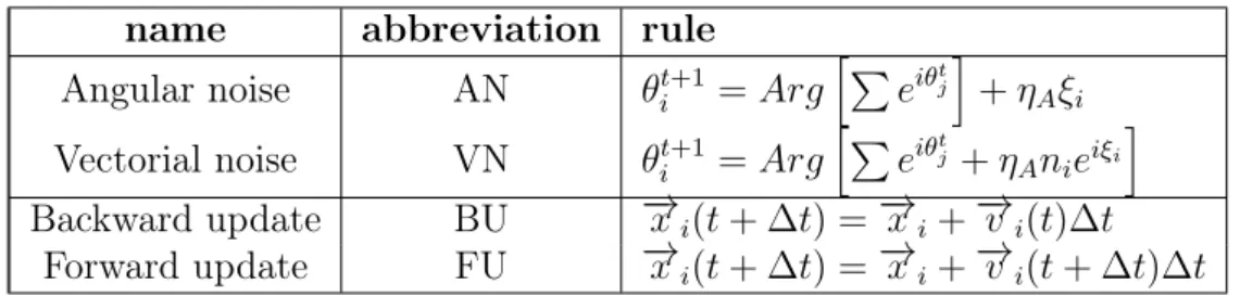
There are several different versions of the model around nowadays, with different ways of adding the noise and with different update rules. Using slightly different variations of the original model has been thought to be ir-relevant to the results, but it has actually led to many conflicting results and a confusion about what type of a phase transition the model has. This confusion was clarified in [23], where the most common versions were clearly defined and compared. The following definitions and notations are taken from that paper, and introduce the two different ways to add noise and the two different update rules, as demonstrated in Table 2.1.

Table 2.1: The different variants of the Vicsek model considered name abbreviation rule

Angular noise AN θt_i+1 =ArghP

eiθtj

i

+ηAξi

Vectorial noise VN θt_i+1 =ArghP

eiθtj₊_η

Anieiξi i

Backward update BU −→xi(t+ ∆t) = →−xi +−→vi(t)∆t

Forward update FU −→xi(t+ ∆t) = −→xi +−→vi(t+ ∆t)∆t

The original Vicsek paper [2] usedangular noise (AN). Using AN consists of determining the angle of motion θ of the ith particle as the average angle of motion of the neighboring j particles, also including i itself. This is then affected by the noise term, which consists of the amplitude of noise ηA and

the uniformly distributed δ-correlated white noiseξ: θt_i+1 =ArghXeiθtj

i

+ηAξi. (2.2)

The AN term can be thought to arise from the error committed by the the unit as it tries to adjust to its neighbors’ average flight direction.

(32)

In [24] it was argued that the noise could also arise from each interac-tion between the ith particle and one of its neighbors. This translates into

vectorial noise (VN):

θ_it+1 =ArghXeiθtj +η

Anieiξi i

. (2.3)

The difference is that the magnitude of AN is independent of the degree of local order, while VN becomes weaker when the local order is increased.

In the original Vicsek paperbackward update(BU) was used. In it one first evaluates the direction of motion and then proceeds to update the position of the particle according to

− →_x

i(t+ ∆t) = −→xi+−→vi(t)∆t. (2.4)

In some newer papers [23] another update rule has been used expecting it to give same results. This method, forward update (FU) is defined as

− →_x

i(t+ ∆t) =−→xi+−→v i(t+ ∆t)∆t. (2.5)

It was shown in [23] that the combination of [AN+BU] yields a second-order phase transition, but the combination of [AN+FU] gives a clear first-order transition. This shows that the update procedure (FU vs BU) may actually influence the results dramatically. Also, the occurrence of first-order transitions are linked to VN and second-order to AN. Clearly, the choice of both update rule and noise affects the results.

2.4.4 Models without an explicit alignment rule

There are also models which do not contain a rule for alignment, but rather portray some collisions between particles in the presence of some interaction potential. One of the simplest models concerning SPPs is a model where the particles are trying to maintain a given absolute velocity and they only interact pairwise through a short-distanced repulsive linear force. This kind of system exhibits collective motion because each of these inelastic collisions between isotropic particles induces alignment, which in turn results in an

(33)

increased overall velocity correlation.

An SPP model where the particles interact only through attraction was considered by Strömbom [27]. He found a variety of patterns, such as swarms (a set of particles with low and varying alignment), undirected mills (a group in which the particles move in a circular path around a common center) and moving aligned groups (in which the units move in a highly aligned manner). Importantly, these structures were stable only in the presence of noise.

2.4.5 The Cucker-Smale model

Exact formulation is a term used for results obtained analytically with a minimum amount of assumptions or approximations concerning the moving particles, except the rules they abide by. Cucker and Smale studied an exact formulation of the convergence to consensus in a population of autonomous agents in [28] and [29]. In their model (CSM) birds, denoted by i= 1, ..., k, are moving in 3 dimensional (Euclidean) space,_R3, trying to reach a common

direction or consensus. The position of the ith bird is given byxi(t)(∈R3).

Every bird adjusts its velocity by adding to it a weighted average of the differences of its velocity with those of other birds. That is, at timet and for bird i vi(t+ 1)−vi(t) = k X j=1 aij(vj(t)−vi(t)) (2.6)

The weights aij quantify the way the birds influence each other, and are

a function of the distance between birds.

Let us define the adjacency matrixA= (aij), where the before-mentioned

element aij measures the ability of birds i and j to communicate with each

other, or their influence on each other. The elements of Ashould take values from the interval (0...1], and the closer unit i is to unit j, the bigger aij

should be (since they exert a stronger influence on each other). β is a tuning parameter affecting the strength of the influence,

aij =

1

(1 +||xi−xj||2)β

, (2.7)

whereβ ≥0. The main benefit of this formulation is that it is a smooth function allowing analytical treatment. The adjacency matrix changes with

(34)

time, since the positions of the birds keep changing with time.

The two main differences between CSM and VM are: 1) the range of interaction is continuous/discontinuous in CSM/VM, and 2) there is noise in VM, but in CSM there is not. In CSM the interaction range is a long-range action decaying with β, while in the VM it has the same intensity for all the neighboring units around a given particle, but only within a well-defined range. Although the two models are related, there are differences in behav-ior that stand out. The adjacency matrix that can be made based on the VM corresponds to a simple graph, whereas the matrix associated with CSM corresponds to a complete weighted graph. In VM convergence to a common direction depends on how the birds are connected to each other, whereas in CSM the weights decrease to zero as birds separate. In CSM the decay is polynomial and converges only with some initial values.

2.4.6 Network and control theoretical models

Networks have been used in recent years to depict the intricate underlying interactions of many a complex system. It has been shown that in many complex systems the number of connections is described by a power law, not a Poissonian distribution as previously thought. [30]

A flock of collectively moving units can be associated with a temporal net-work [5]. In such a netnet-work two units are connected if they interact, and only at the time of the interaction. The complex time evolution of the temporal network can reproduce the effect of moving units and changing environment. This kind of topology is referred to in control theory as a switching topology. Using control theory, we can reformulate the problem of consensus in col-lective motion as follows: given a set of agents, who want to reach an agree-ment, regarding a certain quantity (direction of movement) that depends on the state of the agents. The interaction rule that defines the information exchange between a unit and its neighbors is called the consensus algorithm (or "protocol"). This system can be represented by a graph G = (V, E), in which the agents are the nodes V = 1,2, ..., n. Two nodes are connected with an edge e ∈ E if, and only if, they communicate with each other. In this case they are neighbors. Accordingly, the neighbors of node i are Ni =j ∈V : (i, j)∈E.

(35)

asymp-CHAPTER 2. THEORY 35

totically to an agreement via local communication. Let A = (aij) denote

the adjacency matrix, which defines the communication pattern among the agents: if i and j interact with each other, then aij > 0, otherwise aij = 0.

Notably, in the case of flocks both A and G vary with time, i.e. A = A(t)

and G=G(t) [5].

Assuming a simple protocol, the state of agentican change according to d

dtxi(t) =

X j∈Ni

aij(xj(t)−xi(t)) (2.8)

and hence defines a distributed consensus algorithm, i.e. it asymptoti-cally solves an average-consensus problem for all initial states. In the case of undirected graphs the equation simplifies to the collective decision being the average of the initial state of the nodes. Once the protocol problem has been solved, we know how the system behaves in trying to reach consensus. [31, 32]

2.4.7 Models based on insect behavior

As an example of a 2D model, in [10] it was shown that Mormon cricket and Desert locust individuals with escape and pursuit behavior exhibit collective motion. The escape reaction is triggered in an individual if it is approached from behind by another individual. This causes the individual to increase its speed to avoid being attacked. If the individual notices one of its mates moving away, it increases its velocity in the direction of the fleeing individual, participating in pursuit behavior. Other cases do not trigger any response. According to the simulations, at moderate noise intensity and high particle density, these interactions (pursuit and escape) lead to global collective mo-tion, irrespective of the detailed model parameters.

Another insect collective motion phenomena is the tendency of locusts to suddenly and coherently switch their direction of movement. It has been suggested in [33] that these ergodic directional switches might be the result of small errors made by the insects when trying to mimic the motion of their neighbors. These errors usually cancel each other out, but on a very large time scale the errors might accumulate and produce such a switch in motion. In Figure 2.8 can be seen a swarm of locusts in a lab setting.

(36)

Figure 2.8: A picture from a study of marching locusts. The locusts circle around the container, until suddenly they simultaneously change di-rections. This has been explained by the accumulation of small errors made by the locusts as they try to mimic the motion of their neighbors. Source: http://www.kurzweilai.net/social-networking-for-locusts

(37)

Chapter 3 Methods

3.1 Vicsek model with leaders

In this thesis, I have studied the Vicsek model using angular noise (AN) and backwards update (BU), as was done in the original Vicsek paper [2]. AN consists of calculating the average of all near enough neighbors’ flight direc-tions and adding noise to the result. BU refers to calculating the direction of motion and then updating the position of the unit according to (2.4).

My focus is on controlling the swarm’s direction of movement. To do this I add an additional component: leaders. Leaders are units that don’t obey the normal update rules, but instead keep a constant direction. I study if these leaders can ’hijack’ the flock and make them fly in the same direction as the leaders are flying.This setting has been motivated by the experimental results of [3], as discussed in Section 2.3.3, where it was shown that as few as one trained fish individual could direct the entire fish school to a feeding site without the school breaking up.

In brief, there are N units, of which NL leaders are chosen, that have a

constant flight direction (φ = 0), don’t follow other units, and are unaffected by noise.

As a control parameter, the average flight direction in radians, vavg =

1

N v0

(v1 +v2+...+vN) (3.1)

is recorded at the end of each cycle (i.e. once all units have been updated). v0 is a normalization factor, it’s the VM unit speed. I used v0 = 0.03, as was

done in the original Vicsek paper for the same reasons; using this speed the 37

(38)

CHAPTER 3. METHODS 38

particles always interact with their actual neighbors and move fast enough to change the configuration after a few direction updates.

Noise η is a key factor in VM. Using AN, we can calculate the noise according to (2.2). The density

ρ= N

L2 (3.2)

of the units also affects the behavior of the system. As was stated in the original paper, noise and density decide if flocking behavior is even possible in the system: with high densities and noise the movement is random, with high density and low noise the motion is ordered. With small densities and high noise the particles tend to form groups moving coherently in random directions, and this is manifested in the order parameterφ(eq. (2.1)) attain-ing non-zero values. When most units are movattain-ing in the same direction, the values of φ approach 1.

3.2 Simulations

I wrote my code in Python. The code was based on the original Vicsek algo-rithm, implemented by Paavo Niskala. Initially all the units are distributed randomly, with a random initial flight direction. The amount of leaders was varied and the order parameter ρ, i.e. the average flight direction of all the units was recorded after each cycle. A cycle is defined to be when each unit has been updated once.

To find out the right amount of noise with a certain density used, I re-peated the measures made in the original paper as follows; I take different values of noise and compute the ensemble average of the order parameter corresponding to that value of noise. With small enough values of noise, the order parameter is non-zero and we have flocking behavior.

I then look into the effect of NL on the behavior of the flock. I increase

the amount of leaders and see how much they affect the group’s movements. Without leaders and with a few leaders the movement of the units should be random, and the order parameter should be practically zero. When the amount of leaders increases, the movement of the units as a whole should start indicating ordered movement.

(39)

CHAPTER 3. METHODS 39

Both the systems being investigated and the time frames used are finite. Hence, it must be chosen when the system state is measured and what is interpreted as uni-directional movement. When the different variables and settings are varied, we can better determine what happens in systems of dif-ferent or infinite size. By choosing a specific ending time for the runs, I can define a variable which will tell about the behavior of the units. This binary variable, pL, describes whether the run ended with the flock adopting the

leaders’ flight direction or not. In the time window [t1, t2] the order

param-eter is calculated at the end of each cycle. If ρ is between [−x, x] at every cycle with t ∈[t1, t2], then pL= 1, otherwise pL = 0. This in itself does not

tell a lot, but by using an ensemble approach, we can calculate how many runs m of total M runs end with "hijacking".

After I have shown that leaders do have a great effect on the flock’s movements even when their percentage is small, I go on to see what the critical leader densities

fL,C =

NL,C

N (3.3)

are so that above this limit the flock follows the leaders with a probabil-ity of 1₂. So the critical value is defined as the value above which it is more probable to follow the flock than not.

After calculating the critical values, the effect of system size can be stud-ied. By keeping ρ fixed and varying L and N, the critical leader amount can be plotted against system size. In accordance to Figure 2.3, one would expect the transition to become more and more abrupt with growing system size.

Due to computational restrictions, the normal simulations use t1 = 150,

t2 = 200. The effect of waiting time, i.e. the point at which the simulations

are terminated, can be studied, however. This is done by having the simula-tions run for the maximum time needed (in this case 1250 cycles) and then using the same data to examine the earlier time windows. That is, once we have the data for 1250 cycles, we can use different (t1, t2) pairs and see how

the results change if we terminate the run at different points. This way we can make observations about what might have happened if we’d just let the runs used for earlier experiments continue. To keep the results comparable, the difference t2−t1 is fixed to the value of 50.

(40)

Chapter 4 Results

4.1 Determining the level of noise

η

As was stated in [2], noise and density decide if flocking behavior is possible in a system. To have particles that form groups that move in a flock-like manner, high densities and low levels of noise are needed.

Values ofN andLwere chosen based on a hunch, and then tested whether they led to the desired effect, after which they were fixed. Using N = 500

andL= 25, we get from equation (3.2): ρ= 0.8. Using this density I plot the average velocity as a function ofη to find out when the order parameter gets a non-zero value. When the order parameter, depicting the average direction of movement of the whole system, is non-zero, we know there is flocking be-havior to be detected. The plot can be seen in Figure 4.1. I choose the value η = 0.5as it is clearly in the non-zero area. This noise level is used in all the following simulations, and hence ρis kept constant.

Table 4.1: The parameters used for the flock simulations.

Parameter value used

N (amount of units) 500

NL (amount of leaders) 0-99

L (length of the side of the simulation area) 25 v0 (the speed of the units) 0.03

η (noise) 0.5

(41)

CHAPTER 4. RESULTS 41

0

1

2

3

4

5

6 η

0.0

0.2

0.4

0.6

0.8

1.0 v

a

N = 500 L = 25

Figure 4.1: The order parameter as a function of system noise. Each data point is an ensemble average of 50 runs made. The value η = 0.5 is chosen as it is clearly in the non-zero area.

4.2 The effect of the number of leaders

N

L A series of example runs with NL = 10 can be seen in Fig. 4.2. As time

passes, the units form flocks that mostly move in the direction of the leaders, with some deviance accounted for by the effect of noise. Running simula-tions with the parameters indicated in Table 4.1, we see clear indication of the flock being hijacked by the leaders already with just a couple of leaders. To illustrate this, we can compare the average flight direction as a function of time to the constant flight direction of the leaders. As can be seen in Fig. 4.3, the average flight direction (the blue curve) converges to oscillations around the leader’s flight direction (marked with red). This happens the faster the more leaders there are. The closer the blue curve is to the constant red line, the more the leaders dominate the flight direction. Even with a value of NL = 8, the average flight direction reaches the constant line φ = 0 before

(42)

(a)t= 1 (b)t = 28

(c)t= 100 (d)t = 249

Figure 4.2: An example of how leaders affect the behavior of the flock, with NL = 10. The leaders are marked and circled in red. As time

passes, the birds form flocks which merge into bigger flocks. The leaders take control of the flocks and most birds fly in the direction φ = 0 (with some perturbations due to noise). The black circle shows the range of interaction.

(43)

into a constant direction.

To study the leaders effect more rigorously, the criteria for the complete "hijacking" must be decided. I define this as follows: The flock follows the leaders at the end of the run, if every value of the order parameter at time t ∈[150,200] is between [−₈π,π₈]. I then make runs for different values of NL

and record whether the run ended with the flock following the leader or not, i.e. a binary variable. For each value of NL, I performed 100 runs of the

simulation, and calculated pL, the fraction of runs atNL where the flock was

seen to follow the leaders between t ∈ [150,200]. Thus we get Figure 4.4, which shows that as the amount of leaders increases, the fraction pL grows

monotonically towards 1.

4.3 Varying the system size

N

and the waiting

time

t

I study the effect of both system size and waiting time on flock hijacking, with the intention to use these results to extrapolate to a infinite sized sys-tem. We want to get a general result, by studying the system as it grows towards infinite size but we can also study a finite system with a infinite waiting time. If we get finite results for the amount of leaders in an infinite system, it tells us that we can control huge swarms without the need for immense amounts of leaders.

By keepingρ practically constant, the effects of system size can be stud-ied. The values used for this part are gathered in Table 4.2. By taking the six system sizes and comparing the absolute and relative amounts of leaders we get Figure 4.5. We can see that as the system size grows, the amount of leaders needed to control the flock decreases. For example, where nearly 10% leaders are needed for N = 500, only round 5% are needed when N = 1000. Considering that the percentage of leaders needed goes down as a function of system size, it seems feasible that we can get similar results with a finite system by just waiting long enough. That’s why I also study the effect of the time window chosen, i.e. when the ending check is performed. The base case is the time window t = [150,200] used for all the other simulations. What we want to see is whether waiting longer affects the amount of runs finishing in a leader-controlled state. This was done using a run lasting 1250 cycles,

(44)

CHAPTER 4. RESULTS 44 0 50 100 150 200 250 Time (cycles) −π −3₄π −π2 −π₄ 0 +π 4 +π₂ −34π π Direction (rad) (a)NL = 0 0 50 100 150 200 250 Time (cycles) −π −3₄π −π2 −π₄ 0 +π 4 +π₂ −34π π Direction (rad) (b)NL = 4 0 50 100 150 200 250 Time (cycles) −π −34π −π2 −π4 0 +π 4 +π 2 −34π π Direction (rad) (c) NL = 8 0 50 100 150 200 250 Time (cycles) −π −34π −π2 −π4 0 +π 4 +π 2 −34π π Direction (rad) (d)NL = 74

Figure 4.3: Four examples of the flock’s average flight direction as a function of time, with flock size N being 500. The red line indicates the leaders’ flight direction. The closer the dots are to the red line, the more the units are flying in the same direction as the leaders.

(45)

0

10

20

30

40

50 Amount of leaders

0.0

0.2

0.4

0.6

0.8

1.0 p_L

Figure 4.4: The probability pL that the flock is following the leader

at the end of 200 cycles as a function of the amount of leaders. N = 500, L= 25 and ρ= 0.8. Each data point is an average of 100 runs.

and then checking whether the run had ended using different time windows. Thus we can see how the results of the other tests might have behaved if we had been able to wait longer.

From the size and time plots I determine the critical values of leaders needed for group "hijacking". This choice is rather arbitrary, since the single runs are stochastic in nature and taking the value pL= 1 is not really

sensi-ble. I do this by taking the percentage corresponding to (3.3), pL = 0.5 and

say that this is the corresponding pL,c,N/pL,c,t. These values can be seen in

Table 4.3 and plotted in Figure 4.7. In the same figure we have the inverses of both system size and waiting time plotted against pL,c. This is done so that

we can extrapolate these values to infinity and see whether the percentage of leaders goes to zero. By doing an approximate fit (the red line) to the first values of the curves and reading the point where it intersects the y-axis, we get an estimate for the percentage of leaders needed in an infinite system. As

(46)

Table 4.2: The parameters used for critical simulations.

N L ρ 100 11 0.826 250 18 0.772 500 25 0.800 1000 35 0.816 2000 50 0.800 5000 79 0.801 0 10 20 30 40 50 Amount of leaders 0.0 0.2 0.4 0.6 0.8 1.0 pL N=100 N=250 N=500 N=1000 N=2000 N=5000

(a) Absolute values

0 2 4 6 8 10 Percentage of leaders (%) 0.0 0.2 0.4 0.6 0.8 1.0 pL N=100 N=250 N=500 N=1000 N=2000 N=5000 (b) Relative values

Figure 4.5: The effect of system size on the leader’s and their flock "hijacking".

can be seen from the figure, we get the value of about 0.2% for both varied inverse time and size, which is reasonably within error estimates and can be thought to be zero. This value of 0.2% is, evidently, very close to zero, and it would be interesting to investigate whether, in fact, any non-zero fraction of leaders would be enough to hijack the flock. However, this would require simulations on much larger systems, and is thus beyond the scope of this work.

(47)

0

2

4

6

8

10 Percentage of leaders (%)

0.0

0.2

0.4

0.6

0.8

1.0

pL

t = [150,200]

t = [200,250]

t = [300,350]

t = [600,650]

t = [1200,1250]

Figure 4.6: The effect of waiting time window choice on the "hijack-ing" of the flock. If every value of the order parameter in the time window is between [−₈π,π₈], then the flock has adopted the leader’s flight direction.

Table 4.3: The critical values from the size and time simulations.

N pL,c,N (%) t pL,c,t (%) 100 2.88 t= [150,200] 1.50 250 2.63 t= [200,250] 1.38 500 2.02 t= [300,350] 1.35 1000 1.51 t= [600,650] 0.76 2000 0.75 t= [1200,1250] 0.51 5000 0.50

(48)

CHAPTER 4. RESULTS 48 0 1000 2000 3000 4000 5000 System size 0 0.5 1.0 1.5 2.0 2.5 3.0 pL,c,N (% )

(a) System size

0 200 400 600 800 1000 1200 Waiting time 0 0.2 0.4 0.6 0.8 1.0 1.2 1.4 1.6 pL,c,t (% ) (b) Waiting time 0 0.002 0.004 0.006 0.008 0.01

Inverse system size 1/N

0 0.5 1.0 1.5 2.0 2.5 3.0 pL, c, N (%)

(c) Inverse system size

0 0.001 0.002 0.003 0.004 0.005 0.006 0.007 Inverse waiting time 1/tau (1/cycle)

0 0.2 0.4 0.6 0.8 1.0 1.2 1.4 1.6 pL, c, t (%)

(d) Inverse waiting time

Figure 4.7: The effect of system size and waiting time on the "hi-jacking" of the flock. Clearly the bigger the system and the longer we wait, the less percentage of leaders is needed to steer the entire flock into the direction wanted. The lower pictures show the inverse of both system size and waiting time. By making an approximate fit to the part closest to zero, we can extrapolate to find the probable point where the curve intersects the y-axis. This corresponds to the ideal limit N(τ)→ ∞,_N1(1_τ)→0. In reality the value for both is about 0.2%.

Kollektiivisen liikkeen ohjaaminen

Steering collective motion

Preface

Symbols

Abbreviations

Contents

List of Tables

List of Figures

Chapter 1

Introduction

Chapter 2

Theory

2.1

Collective motion - basics

2.2

The physics of collective motion

2.3

Observations and experiments

2.3.1

Inanimate objects

2.3.2

Insects

2.3.3

Fish

2.3.4

Birds

2.3.5

Mammals

2.3.6

Robots

2.4

Models and simulations

2.4.1

A quick look at agent-based modeling

2.4.2

Precursors: The Reynolds and Aoki models

2.4.3

The Vicsek model

2.4.4

Models without an explicit alignment rule

2.4.5

The Cucker-Smale model

2.4.6

Network and control theoretical models

2.4.7

Models based on insect behavior

Chapter 3

Methods

3.1

Vicsek model with leaders

3.2

Simulations

Chapter 4

Results

4.1

Determining the level of noise

η

0

1

2

3

4

5

6

η

0.0

0.2

0.4

0.6

0.8

1.0

v

N = 500 L = 25

4.2

The effect of the number of leaders

N

4.3

Varying the system size

N

and the waiting