To my parents
CONTENTS
PREFACE ... xvii
FREQUENTLY USED SYMBOLS AND ABBREVIATIONS... xxi
CHAPTER 1 INTRODUCTION...1
1.1 Signals and Information ...2
1.2 Signal Processing Methods ...3
1.2.1 Non−parametric Signal Processing ...3
1.2.2 Model-Based Signal Processing ...4
1.2.3 Bayesian Statistical Signal Processing ...4
1.2.4 Neural Networks...5
1.3 Applications of Digital Signal Processing ...5
1.3.1 Adaptive Noise Cancellation and Noise Reduction ...5
1.3.2 Blind Channel Equalisation...8
1.3.3 Signal Classification and Pattern Recognition ...9
1.3.4 Linear Prediction Modelling of Speech...11
1.3.5 Digital Coding of Audio Signals ...12
1.3.6 Detection of Signals in Noise ...14
1.3.7 Directional Reception of Waves: Beam-forming ...16
1.3.8 Dolby Noise Reduction ...18
1.3.9 Radar Signal Processing: Doppler Frequency Shift ...19
1.4 Sampling and Analog–to–Digital Conversion ...21
1.4.1 Time-Domain Sampling and Reconstruction of Analog Signals ...22
1.4.2 Quantisation...25
Bibliography...27
CHAPTER 2 NOISE AND DISTORTION...29
2.1 Introduction...30
2.2 White Noise ...31
2.3 Coloured Noise ...33
2.4 Impulsive Noise ...34
2.5 Transient Noise Pulses...35
viii Contents
2.7 Shot Noise...38
2.8 Electromagnetic Noise ...38
2.9 Channel Distortions ...39
2.10 Modelling Noise ...40
2.10.1 Additive White Gaussian Noise Model (AWGN)...42
2.10.2 Hidden Markov Model for Noise ...42
Bibliography...43
CHAPTER 3 PROBABILITY MODELS ...44
3.1 Random Signals and Stochastic Processes ...45
3.1.1 Stochastic Processes ...47
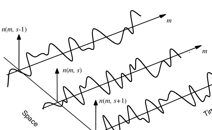
3.1.2 The Space or Ensemble of a Random Process ...47
3.2 Probabilistic Models ...48
3.2.1 Probability Mass Function (pmf)...49
3.2.2 Probability Density Function (pdf)...50
3.3 Stationary and Non-Stationary Random Processes...53
3.3.1 Strict-Sense Stationary Processes...55
3.3.2 Wide-Sense Stationary Processes...56
3.3.3 Non-Stationary Processes ...56
3.4 Expected Values of a Random Process...57
3.4.1 The Mean Value ...58
3.4.2 Autocorrelation...58
3.4.3 Autocovariance...59
3.4.4 Power Spectral Density ...60
3.4.5 Joint Statistical Averages of Two Random Processes...62
3.4.6 Cross-Correlation and Cross-Covariance ...62
3.4.7 Cross-Power Spectral Density and Coherence ...64
3.4.8 Ergodic Processes and Time-Averaged Statistics ...64
3.4.9 Mean-Ergodic Processes ...65
3.4.10 Correlation-Ergodic Processes ...66
3.5 Some Useful Classes of Random Processes ...68
3.5.1 Gaussian (Normal) Process ...68
3.5.2 Multivariate Gaussian Process ...69
3.5.3 Mixture Gaussian Process ...71
3.5.4 A Binary-State Gaussian Process ...72
3.5.5 Poisson Process ...73
3.5.6 Shot Noise ...75
3.5.7 Poisson–Gaussian Model for Clutters and Impulsive Noise...77
3.5.8 Markov Processes...77
Contents ix
3.6 Transformation of a Random Process...81
3.6.1 Monotonic Transformation of Random Processes ...81
3.6.2 Many-to-One Mapping of Random Signals ...84
3.7 Summary...86
Bibliography...87
CHAPTER 4 BAYESIAN ESTIMATION...89
4.1 Bayesian Estimation Theory: Basic Definitions ...90
4.1.1 Dynamic and Probability Models in Estimation...91
4.1.2 Parameter Space and Signal Space...92
4.1.3 Parameter Estimation and Signal Restoration ...93
4.1.4 Performance Measures and Desirable Properties of Estimators ...94
4.1.5 Prior and Posterior Spaces and Distributions ...96
4.2 Bayesian Estimation...100
4.2.1 Maximum A Posteriori Estimation ...101
4.2.2 Maximum-Likelihood Estimation ...102
4.2.3 Minimum Mean Square Error Estimation ...105
4.2.4 Minimum Mean Absolute Value of Error Estimation...107
4.2.5 Equivalence of the MAP, ML, MMSE and MAVE for Gaussian Processes With Uniform Distributed Parameters ...108
4.2.6 The Influence of the Prior on Estimation Bias and Variance...109
4.2.7 The Relative Importance of the Prior and the Observation...113
4.3 The Estimate–Maximise (EM) Method ...117
4.3.1 Convergence of the EM Algorithm ...118
4.4 Cramer–Rao Bound on the Minimum Estimator Variance...120
4.4.1 Cramer–Rao Bound for Random Parameters ...122
4.4.2 Cramer–Rao Bound for a Vector Parameter...123
4.5 Design of Mixture Gaussian Models ...124
4.5.1 The EM Algorithm for Estimation of Mixture Gaussian Densities ...125
4.6 Bayesian Classification ...127
4.6.1 Binary Classification ...129
4.6.2 Classification Error...131
4.6.3 Bayesian Classification of Discrete-Valued Parameters .132 4.6.4 Maximum A Posteriori Classification...133
4.6.5 Maximum-Likelihood (ML) Classification...133
4.6.6 Minimum Mean Square Error Classification ...134
x Contents 4.6.8 Bayesian Estimation of the Most Likely State
Sequence...136
4.7 Modelling the Space of a Random Process...138
4.7.1 Vector Quantisation of a Random Process...138
4.7.2 Design of a Vector Quantiser: K-Means Clustering...138
4.8 Summary...140
Bibliography...141
CHAPTER 5 HIDDEN MARKOV MODELS...143
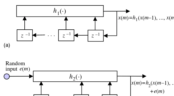
5.1 Statistical Models for Non-Stationary Processes ...144
5.2 Hidden Markov Models ...146
5.2.1 A Physical Interpretation of Hidden Markov Models ...148
5.2.2 Hidden Markov Model as a Bayesian Model ...149
5.2.3 Parameters of a Hidden Markov Model ...150
5.2.4 State Observation Models ...150
5.2.5 State Transition Probabilities ...152
5.2.6 State–Time Trellis Diagram ...153
5.3 Training Hidden Markov Models ...154
5.3.1 Forward–Backward Probability Computation...155
5.3.2 Baum–Welch Model Re-Estimation ...157
5.3.3 Training HMMs with Discrete Density Observation Models ...159
5.3.4 HMMs with Continuous Density Observation Models ...160
5.3.5 HMMs with Mixture Gaussian pdfs...161
5.4 Decoding of Signals Using Hidden Markov Models ...163
5.4.1 Viterbi Decoding Algorithm...165
5.5 HMM-Based Estimation of Signals in Noise...167
5.6 Signal and Noise Model Combination and Decomposition...170
5.6.1 Hidden Markov Model Combination ...170
5.6.2 Decomposition of State Sequences of Signal and Noise.171 5.7 HMM-Based Wiener Filters ...172
5.7.1 Modelling Noise Characteristics ...174
5.8 Summary...174
Bibliography...175
CHAPTER 6 WIENER FILTERS...178
6.1 Wiener Filters: Least Square Error Estimation ...179
Contents xi
6.3 Interpretation of Wiener Filters as Projection in Vector Space ...187
6.4 Analysis of the Least Mean Square Error Signal ...189
6.5 Formulation of Wiener Filters in the Frequency Domain...191
6.6 Some Applications of Wiener Filters...192
6.6.1 Wiener Filter for Additive Noise Reduction ...193
6.6.2 Wiener Filter and the Separability of Signal and Noise ..195
6.6.3 The Square-Root Wiener Filter ...196
6.6.4 Wiener Channel Equaliser...197
6.6.5 Time-Alignment of Signals in Multichannel/Multisensor Systems...198
6.6.6 Implementation of Wiener Filters ...200
6.7 The Choice of Wiener Filter Order ...201
6.8 Summary...202
Bibliography...202
CHAPTER 7 ADAPTIVE FILTERS...205
7.1 State-Space Kalman Filters...206
7.2 Sample-Adaptive Filters ...212
7.3 Recursive Least Square (RLS) Adaptive Filters ...213
7.4 The Steepest-Descent Method ...219
7.5 The LMS Filter ...222
7.6 Summary...224
Bibliography...225
CHAPTER 8 LINEAR PREDICTION MODELS ...227
8.1 Linear Prediction Coding...228
8.1.1 Least Mean Square Error Predictor ...231
8.1.2 The Inverse Filter: Spectral Whitening ...234
8.1.3 The Prediction Error Signal...236
8.2 Forward, Backward and Lattice Predictors ...236
8.2.1 Augmented Equations for Forward and Backward Predictors...239
8.2.2 Levinson–Durbin Recursive Solution ...239
8.2.3 Lattice Predictors...242
8.2.4 Alternative Formulations of Least Square Error Prediction...244
8.2.5 Predictor Model Order Selection...245
xii Contents
8.4 MAP Estimation of Predictor Coefficients ...249
8.4.1 Probability Density Function of Predictor Output...249
8.4.2 Using the Prior pdf of the Predictor Coefficients ...251
8.5 Sub-Band Linear Prediction Model ...252
8.6 Signal Restoration Using Linear Prediction Models...254
8.6.1 Frequency-Domain Signal Restoration Using Prediction Models ...257
8.6.2 Implementation of Sub-Band Linear Prediction Wiener Filters...259
8.7 Summary...261
Bibliography...261
CHAPTER 9 POWER SPECTRUM AND CORRELATION ...263
9.1 Power Spectrum and Correlation ...264
9.2 Fourier Series: Representation of Periodic Signals ...265
9.3 Fourier Transform: Representation of Aperiodic Signals...267
9.3.1 Discrete Fourier Transform (DFT) ...269
9.3.2 Time/Frequency Resolutions, The Uncertainty Principle ...269
9.3.3 Energy-Spectral Density and Power-Spectral Density ....270
9.4 Non-Parametric Power Spectrum Estimation ...272
9.4.1 The Mean and Variance of Periodograms ...272
9.4.2 Averaging Periodograms (Bartlett Method) ...273
9.4.3 Welch Method: Averaging Periodograms from Overlapped and Windowed Segments...274
9.4.4 Blackman–Tukey Method ...276
9.4.5 Power Spectrum Estimation from Autocorrelation of Overlapped Segments ...277
9.5 Model-Based Power Spectrum Estimation ...278
9.5.1 Maximum–Entropy Spectral Estimation ...279
9.5.2 Autoregressive Power Spectrum Estimation ...282
9.5.3 Moving-Average Power Spectrum Estimation...283
9.5.4 Autoregressive Moving-Average Power Spectrum Estimation...284
9.6 High-Resolution Spectral Estimation Based on Subspace Eigen-Analysis ...284
9.6.1 Pisarenko Harmonic Decomposition...285
9.6.2 Multiple Signal Classification (MUSIC) Spectral Estimation...288
Contents xiii
9.7 Summary...294
Bibliography...294
CHAPTER 10 INTERPOLATION...297
10.1 Introduction...298
10.1.1 Interpolation of a Sampled Signal ...298
10.1.2 Digital Interpolation by a Factor of I...300
10.1.3 Interpolation of a Sequence of Lost Samples ...301
10.1.4 The Factors That Affect Interpolation Accuracy...303
10.2 Polynomial Interpolation...304
10.2.1 Lagrange Polynomial Interpolation ...305
10.2.2 Newton Polynomial Interpolation ...307
10.2.3 Hermite Polynomial Interpolation ...309
10.2.4 Cubic Spline Interpolation...310
10.3 Model-Based Interpolation ...313
10.3.1 Maximum A Posteriori Interpolation ...315
10.3.2 Least Square Error Autoregressive Interpolation ...316
10.3.3 Interpolation Based on a Short-Term Prediction Model ...317
10.3.4 Interpolation Based on Long-Term and Short-term Correlations ...320
10.3.5 LSAR Interpolation Error...323
10.3.6 Interpolation in Frequency–Time Domain ...326
10.3.7 Interpolation Using Adaptive Code Books...328
10.3.8 Interpolation Through Signal Substitution ...329
10.4 Summary...330
Bibliography...331
CHAPTER 11 SPECTRAL SUBTRACTION...333
11.1 Spectral Subtraction ...334
11.1.1 Power Spectrum Subtraction ...337
11.1.2 Magnitude Spectrum Subtraction ...338
11.1.3 Spectral Subtraction Filter: Relation to Wiener Filters .339 11.2 Processing Distortions ...340
11.2.1 Effect of Spectral Subtraction on Signal Distribution...342
11.2.2 Reducing the Noise Variance ...343
11.2.3 Filtering Out the Processing Distortions ...344
11.3 Non-Linear Spectral Subtraction ...345
11.4 Implementation of Spectral Subtraction ...348
xiv Contents
11.5 Summary...352
Bibliography...352
CHAPTER 12 IMPULSIVE NOISE ...355
12.1 Impulsive Noise ...356
12.1.1 Autocorrelation and Power Spectrum of Impulsive Noise ...359
12.2 Statistical Models for Impulsive Noise...360
12.2.1 Bernoulli–Gaussian Model of Impulsive Noise ...360
12.2.2 Poisson–Gaussian Model of Impulsive Noise...362
12.2.3 A Binary-State Model of Impulsive Noise ...362
12.2.4 Signal to Impulsive Noise Ratio...364
12.3 Median Filters ...365
12.4 Impulsive Noise Removal Using Linear Prediction Models ...366
12.4.1 Impulsive Noise Detection ...367
12.4.2 Analysis of Improvement in Noise Detectability ...369
12.4.3 Two-Sided Predictor for Impulsive Noise Detection ....372
12.4.4 Interpolation of Discarded Samples ...372
12.5 Robust Parameter Estimation...373
12.6 Restoration of Archived Gramophone Records ...375
12.7 Summary...376
Bibliography...377
CHAPTER 13 TRANSIENT NOISE PULSES...378
13.1 Transient Noise Waveforms ...379
13.2 Transient Noise Pulse Models ...381
13.2.1 Noise Pulse Templates ...382
13.2.2 Autoregressive Model of Transient Noise Pulses ...383
13.2.3 Hidden Markov Model of a Noise Pulse Process...384
13.3 Detection of Noise Pulses ...385
13.3.1 Matched Filter for Noise Pulse Detection ...386
13.3.2 Noise Detection Based on Inverse Filtering ...388
13.3.3 Noise Detection Based on HMM ...388
13.4 Removal of Noise Pulse Distortions ...389
13.4.1 Adaptive Subtraction of Noise Pulses ...389
13.4.2 AR-based Restoration of Signals Distorted by Noise Pulses ...392
Contents xv
Bibliography...395
CHAPTER 14 ECHO CANCELLATION ...396
14.1 Introduction: Acoustic and Hybrid Echoes ...397
14.2 Telephone Line Hybrid Echo ...398
14.3 Hybrid Echo Suppression ...400
14.4 Adaptive Echo Cancellation ...401
14.4.1 Echo Canceller Adaptation Methods...403
14.4.2 Convergence of Line Echo Canceller ...404
14.4.3 Echo Cancellation for Digital Data Transmission...405
14.5 Acoustic Echo ...406
14.6 Sub-Band Acoustic Echo Cancellation...411
14.7 Summary...413
Bibliography...413
CHAPTER 15 CHANNEL EQUALIZATION AND BLIND DECONVOLUTION...416
15.1 Introduction...417
15.1.1 The Ideal Inverse Channel Filter ...418
15.1.2 Equalization Error, Convolutional Noise ...419
15.1.3 Blind Equalization...420
15.1.4 Minimum- and Maximum-Phase Channels...423
15.1.5 Wiener Equalizer...425
15.2 Blind Equalization Using Channel Input Power Spectrum...427
15.2.1 Homomorphic Equalization ...428
15.2.2 Homomorphic Equalization Using a Bank of High- Pass Filters ...430
15.3 Equalization Based on Linear Prediction Models...431
15.3.1 Blind Equalization Through Model Factorisation...433
15.4 Bayesian Blind Deconvolution and Equalization ...435
15.4.1 Conditional Mean Channel Estimation ...436
15.4.2 Maximum-Likelihood Channel Estimation...436
15.4.3 Maximum A Posteriori Channel Estimation ...437
15.4.4 Channel Equalization Based on Hidden Markov Models...438
15.4.5 MAP Channel Estimate Based on HMMs...441
15.4.6 Implementations of HMM-Based Deconvolution ...442
xvi Contents
15.5.1 LMS Blind Equalization...448
15.5.2 Equalization of a Binary Digital Channel...451
15.6 Equalization Based on Higher-Order Statistics ...453
15.6.1 Higher-Order Moments, Cumulants and Spectra ...454
15.6.2 Higher-Order Spectra of Linear Time-Invariant Systems ...457
15.6.3 Blind Equalization Based on Higher-Order Cepstra ...458
15.7 Summary...464
Bibliography...465
INDEX ...467
PREFACE
Signal processing theory plays an increasingly central role in the development of modern telecommunication and information processing systems, and has a wide range of applications in multimedia technology, audio-visual signal processing, cellular mobile communication, adaptive network management, radar systems, pattern analysis, medical signal processing, financial data forecasting, decision making systems, etc. The theory and application of signal processing is concerned with the identification, modelling and utilisation of patterns and structures in a signal process. The observation signals are often distorted, incomplete and noisy. Hence, noise reduction and the removal of channel distortion is an important part of a signal processing system. The aim of this book is to provide a coherent and structured presentation of the theory and applications of statistical signal processing and noise reduction methods.
This book is organised in 15 chapters.
Chapter 1 begins with an introduction to signal processing, and provides a brief review of signal processing methodologies and applications. The basic operations of sampling and quantisation are reviewed in this chapter.
Chapter 2 provides an introduction to noise and distortion. Several different types of noise, including thermal noise, shot noise, acoustic noise, electromagnetic noise and channel distortions, are considered. The chapter concludes with an introduction to the modelling of noise processes.
Chapter 3 provides an introduction to the theory and applications of probability models and stochastic signal processing. The chapter begins with an introduction to random signals, stochastic processes, probabilistic models and statistical measures. The concepts of stationary, non-stationary and ergodic processes are introduced in this chapter, and some important classes of random processes, such as Gaussian, mixture Gaussian, Markov chains and Poisson processes, are considered. The effects of transformation of a signal on its statistical distribution are considered.
xviii Preface Chapter 5 considers hidden Markov models (HMMs) for non-stationary signals. The chapter begins with an introduction to the modelling of non-stationary signals and then concentrates on the theory and applications of hidden Markov models. The hidden Markov model is introduced as a Bayesian model, and methods of training HMMs and using them for decoding and classification are considered. The chapter also includes the application of HMMs in noise reduction.
Chapter 6 considers Wiener Filters. The least square error filter is formulated first through minimisation of the expectation of the squared error function over the space of the error signal. Then a block-signal formulation of Wiener filters and a vector space interpretation of Wiener filters are considered. The frequency response of the Wiener filter is derived through minimisation of mean square error in the frequency domain. Some applications of the Wiener filter are considered, and a case study of the Wiener filter for removal of additive noise provides useful insight into the operation of the filter.
Chapter 7 considers adaptive filters. The chapter begins with the state-space equation for Kalman filters. The optimal filter coefficients are derived using the principle of orthogonality of the innovation signal. The recursive least squared (RLS) filter, which is an exact sample-adaptive implementation of the Wiener filter, is derived in this chapter. Then the steepest−descent search method for the optimal filter is introduced. The chapter concludes with a study of the LMS adaptive filters.
Chapter 8 considers linear prediction and sub-band linear prediction models. Forward prediction, backward prediction and lattice predictors are studied. This chapter introduces a modified predictor for the modelling of the short−term and the pitch period correlation structures. A maximum a posteriori (MAP) estimate of a predictor model that includes the prior probability density function of the predictor is introduced. This chapter concludes with the application of linear prediction in signal restoration.
Chapter 9 considers frequency analysis and power spectrum estimation. The chapter begins with an introduction to the Fourier transform, and the role of the power spectrum in identification of patterns and structures in a signal process. The chapter considers non−parametric spectral estimation, model-based spectral estimation, the maximum entropy method, and high−
resolution spectral estimation based on eigenanalysis.
Preface xix categories: polynomial and statistical interpolators. A general form of polynomial interpolation as well as its special forms (Lagrange, Newton, Hermite and cubic spline interpolators) are considered. Statistical interpolators in this chapter include maximum a posteriori interpolation, least squared error interpolation based on an autoregressive model, time−frequency interpolation, and interpolation through search of an adaptive codebook for the best signal.
Chapter 11 considers spectral subtraction. A general form of spectral subtraction is formulated and the processing distortions that result form spectral subtraction are considered. The effects of processing-distortions on the distribution of a signal are illustrated. The chapter considers methods for removal of the distortions and also non-linear methods of spectral subtraction. This chapter concludes with an implementation of spectral subtraction for signal restoration.
Chapters 12 and 13 cover the modelling, detection and removal of impulsive noise and transient noise pulses. In Chapter 12, impulsive noise is modelled as a binary−state non-stationary process and several stochastic models for impulsive noise are considered. For removal of impulsive noise, median filters and a method based on a linear prediction model of the signal process are considered. The materials in Chapter 13 closely follow Chapter 12. In Chapter 13, a template-based method, an HMM-based method and an AR model-based method for removal of transient noise are considered.
Chapter 14 covers echo cancellation. The chapter begins with an introduction to telephone line echoes, and considers line echo suppression and adaptive line echo cancellation. Then the problem of acoustic echoes and acoustic coupling between loudspeaker and microphone systems are considered. The chapter concludes with a study of a sub-band echo cancellation system
Chapter 15 is on blind deconvolution and channel equalisation. This chapter begins with an introduction to channel distortion models and the ideal channel equaliser. Then the Wiener equaliser, blind equalisation using the channel input power spectrum, blind deconvolution based on linear predictive models, Bayesian channel equalisation, and blind equalisation for digital communication channels are considered. The chapter concludes with equalisation of maximum phase channels using higher-order statistics.
FREQUENTLY USED SYMBOLS AND ABBREVIATIONS
AWGN Additive white Gaussian noise
ARMA Autoregressive moving average process
AR Autoregressive process
A Matrix of predictor coefficients
ak Linear predictor coefficients
a Linear predictor coefficients vector
aij Probability of transition from state i to state j in a Markov model
αi(t) Forward probability in an HMM
bps Bits per second
b(m) Backward prediction error b(m) Binary state signal
βi(t) Backward probability in an HMM
cxx(m) Covariance of signal x(m)
) , , ,
( 1 2 N
XX k k k
c kth order cumulant of x(m)
) , , ,
( 1 2 k−1
XX
C ω ω ω kth order cumulant spectra of x(m)
D Diagonal matrix
e(m) Estimation error
E[x]
Expectation of xf Frequency variable
) (x
X
f Probability density function for process X
) , ( ,Y x y X
f Joint probability density function of X and Y
) (x y
Y X
f Probability density function of X conditioned on
Y
) ; ( ;Θ xθ
X
f Probability density function of X with θ as a parameter
) , ( ,M xs M S
X
f Probability density function of X given a state sequence s of an HMM M of the process X Φ(m,m–1) State transition matrix in Kalman filter
h Filter coefficient vector, Channel response
hmax Maximum−phase channel response
hmin Minimum−phase channel response
hinv Inverse channel response
xxii Frequently Used Symbols and Abbreviations Hinv(f) Inverse channel frequency response
H Observation matrix, Distortion matrix
I Identity matrix
J Fisher’s information matrix
| J | Jacobian of a transformation
K(m) Kalman gain matrix
LSE Least square error
LSAR Least square AR interpolation
λ Eigenvalue
Λ Diagonal matrix of eigenvalues
MAP Maximum a posterior estimate
MA Moving average process
ML Maximum likelihood estimate
MMSE Minimum mean squared error estimate
m Discrete time index
mk kth order moment
M
A model, e.g. an HMMµ Adaptation convergence factor
µx Expected mean of vector x
n(m) Noise
n(m) A noise vector of N samples
ni(m) Impulsive noise
N(f) Noise spectrum
N*(f) Complex conjugate of N(f)
) (f
N Time-averaged noise spectrum
N
(x,µxx,Σxx) A Gaussian pdf with mean vector µxx and covariance matrix ΣxxO(· ) In the order of (· )
P Filter order (length)
pdf Probability density function
pmf Probability mass function
) ( i
PX x Probability mass function of xi
) , ( , i j
PXY x y Joint probability mass function of xi and yj
(
i j)
PXY x y Conditional probability mass function of xi given
yj
Frequently Used Symbols and Abbreviations xxiii PXY(f) Cross−power spectrum of signals x(m) and y(m)
θ Parameter vector
ˆ
θ Estimate of the parameter vector θ
rk Reflection coefficients
rxx(m) Autocorrelation function
) (m xx
r Autocorrelation vector
Rxx Autocorrelation matrix of signal x(m)
Rxy Cross−correlation matrix
s State sequence
sML Maximum−likelihood state sequence
SNR Signal-to-noise ratio
SINR Signal-to-impulsive noise ratio
σn2 Variance of noise n(m)
Σnn Covariance matrix of noise n(m)
Σxx Covariance matrix of signal x(m)
σx2 Variance of signal x(m)
σn2 Variance of noise n(m)
x(m) Clean signal
ˆ
x (m) Estimate of clean signal
x(m) Clean signal vector
X(f) Frequency spectrum of signal x(m)
X*(f) Complex conjugate of X(f)
) (f
X Time-averaged frequency spectrum of x(m)
X(f,t) Time-frequency spectrum of x(m)
X Clean signal matrix
XH Hermitian transpose of X
y(m) Noisy signal
y(m) Noisy signal vector
ˆ
y (m m −i) Prediction of y(m) based on observations up to time m–i
Y Noisy signal matrix
YH Hermitian transpose of Y
Var Variance
wk Wiener filter coefficients
w(m) Wiener filter coefficients vector
W(f) Wiener filter frequency response
1
INTRODUCTION
1.1 Signals and Information 1.2 Signal Processing Methods
1.3 Applications of Digital Signal Processing 1.4 Sampling and Analog−to−Digital Conversion
ignal processing is concerned with the modelling, detection, identification and utilisation of patterns and structures in a signal process. Applications of signal processing methods include audio hi-fi, digital TV and radio, cellular mobile phones, voice recognition, vision, radar, sonar, geophysical exploration, medical electronics, and in general any system that is concerned with the communication or processing of information. Signal processing theory plays a central role in the development of digital telecommunication and automation systems, and in efficient and optimal transmission, reception and decoding of information. Statistical signal processing theory provides the foundations for modelling the distribution of random signals and the environments in which the signals propagate. Statistical models are applied in signal processing, and in decision-making systems, for extracting information from a signal that may be noisy, distorted or incomplete. This chapter begins with a definition of signals, and a brief introduction to various signal processing methodologies. We consider several key applications of digital signal processing in adaptive noise reduction, channel equalisation, pattern classification/recognition, audio signal coding, signal detection, spatial processing for directional reception of signals, Dolby noise reduction and radar. The chapter concludes with an introduction to sampling and conversion of continuous-time signals to digital signals.
S
H E LL O Advanced Digital Signal Processing and Noise Reduction, Second Edition.
2 Introduction
1.1 Signals and Information
A signal can be defined as the variation of a quantity by which information is conveyed regarding the state, the characteristics, the composition, the trajectory, the course of action or the intention of the signal source. A signal is a means to convey information. The information conveyed in a signal may be used by humans or machines for communication, forecasting, decision-making, control, exploration etc. Figure 1.1 illustrates an information source followed by a system for signalling the information, a communication channel for propagation of the signal from the transmitter to the receiver, and a signal processing unit at the receiver for extraction of the information from the signal. In general, there is a mapping operation that maps the information I(t) to the signal x(t) that carries the information, this mapping function may be denoted as T[· ]and expressed as
)] ( [ ) (t T I t
x = (1.1)
For example, in human speech communication, the voice-generating mechanism provides a means for the talker to map each word into a distinct acoustic speech signal that can propagate to the listener. To communicate a word w, the talker generates an acoustic signal realisation of the word; this acoustic signal x(t) may be contaminated by ambient noise and/or distorted by a communication channel, or impaired by the speaking abnormalities of the talker, and received as the noisy and distorted signal y(t). In addition to conveying the spoken word, the acoustic speech signal has the capacity to convey information on the speaking characteristic, accent and the emotional state of the talker. The listener extracts these information by processing the signal y(t).
In the past few decades, the theory and applications of digital signal processing have evolved to play a central role in the development of modern telecommunication and information technology systems.
Signal processing methods are central to efficient communication, and to the development of intelligent man/machine interfaces in such areas as
Information source
Information to signal mapping
Signal Digital Signal
Processor Channel
Noise
Noisy
signal Signal & Information
Signal Processing Methods 3
speech and visual pattern recognition for multimedia systems. In general, digital signal processing is concerned with two broad areas of information theory:
(a) efficient and reliable coding, transmission, reception, storage and representation of signals in communication systems, and
(b) the extraction of information from noisy signals for pattern recognition, detection, forecasting, decision-making, signal enhancement, control, automation etc.
In the next section we consider four broad approaches to signal processing problems.
1.2 Signal Processing Methods
Signal processing methods have evolved in algorithmic complexity aiming for optimal utilisation of the information in order to achieve the best performance. In general the computational requirement of signal processing methods increases, often exponentially, with the algorithmic complexity. However, the implementation cost of advanced signal processing methods has been offset and made affordable by the consistent trend in recent years of a continuing increase in the performance, coupled with a simultaneous decrease in the cost, of signal processing hardware.
Depending on the method used, digital signal processing algorithms can be categorised into one or a combination of four broad categories. These are non−parametric signal processing, model-based signal processing, Bayesian statistical signal processing and neural networks. These methods are briefly described in the following.
1.2.1 Non−parametric Signal Processing
4 Introduction
improvement in performance. Some examples of non−parametric methods include digital filtering and transform-based signal processing methods such as the Fourier analysis/synthesis relations and the discrete cosine transform. Some non−parametric methods of power spectrum estimation, interpolation and signal restoration are described in Chapters 9, 10 and 11.
1.2.2 Model-Based Signal Processing
Model-based signal processing methods utilise a parametric model of the signal generation process. The parametric model normally describes the predictable structures and the expected patterns in the signal process, and can be used to forecast the future values of a signal from its past trajectory. Model-based methods normally outperform non−parametric methods, since they utilise more information in the form of a model of the signal process. However, they can be sensitive to the deviations of a signal from the class of signals characterised by the model. The most widely used parametric model is the linear prediction model, described in Chapter 8. Linear prediction models have facilitated the development of advanced signal processing methods for a wide range of applications such as low−bit−rate speech coding in cellular mobile telephony, digital video coding, high−resolution spectral analysis, radar signal processing and speech recognition.
1.2.3 Bayesian Statistical Signal Processing
Applications of Digital Signal Processing 5
1.2.4 Neural Networks
Neural networks are combinations of relatively simple non-linear adaptive processing units, arranged to have a structural resemblance to the transmission and processing of signals in biological neurons. In a neural network several layers of parallel processing elements are interconnected with a hierarchically structured connection network. The connection weights are trained to perform a signal processing function such as prediction or classification. Neural networks are particularly useful in non-linear partitioning of a signal space, in feature extraction and pattern recognition, and in decision-making systems. In some hybrid pattern recognition systems neural networks are used to complement Bayesian inference methods. Since the main objective of this book is to provide a coherent presentation of the theory and applications of statistical signal processing, neural networks are not discussed in this book.
1.3 Applications of Digital Signal Processing
In recent years, the development and commercial availability of increasingly powerful and affordable digital computers has been accompanied by the development of advanced digital signal processing algorithms for a wide variety of applications such as noise reduction, telecommunication, radar, sonar, video and audio signal processing, pattern recognition, geophysics explorations, data forecasting, and the processing of large databases for the identification extraction and organisation of unknown underlying structures and patterns. Figure 1.2 shows a broad categorisation of some DSP applications. This section provides a review of several key applications of digital signal processing methods.
1.3.1 Adaptive Noise Cancellation and Noise Reduction
In speech communication from a noisy acoustic environment such as a moving car or train, or over a noisy telephone channel, the speech signal is observed in an additive random noise. In signal measurement systems the information-bearing signal is often contaminated by noise from its surrounding environment. The noisy observation y(m) can be modelled as
6 Introduction
where x(m) and n(m) are the signal and the noise, and m is the discrete-time index. In some situations, for example when using a mobile telephone in a moving car, or when using a radio communication device in an aircraft cockpit, it may be possible to measure and estimate the instantaneous amplitude of the ambient noise using a directional microphone. The signal x(m) may then be recovered by subtraction of an estimate of the noise from the noisy signal.
Figure 1.3 shows a two-input adaptive noise cancellation system for enhancement of noisy speech. In this system a directional microphone takes
DSP Applications
Information Transmission/Storage/Retrieval Information extraction
Signal Classification
Speech recognition, image and character recognition, signal detection
Parameter Estimation
Spectral analysis, radar and sonar signal processing, signal enhancement, geophysics exploration Channel Equalisation
Source/Channel Coding
Speech coding, image coding, data compression, communication over noisy channels
Signal and data communication on adverse channels
Figure 1.2 A classification of the applications of digital signal processing.
y(m)= x(m) +n(m)
α n(m+τ)
x(m)^
n(m)
^ z . . . z
Noise Estimation Filter Noisy signal
Noise
Noise estimate
Signal
Adaptation algorithm
z–1
w2
w1
w0 wP-1
–1 –1
Applications of Digital Signal Processing 7
as input the noisy signal x(m)+n(m) , and a second directional microphone, positioned some distance away, measures the noise αn(m+ τ). The attenuation factor α and the time delay τ provide a rather over-simplified model of the effects of propagation of the noise to different positions in the space where the microphones are placed. The noise from the second microphone is processed by an adaptive digital filter to make it equal to the noise contaminating the speech signal, and then subtracted from the noisy signal to cancel out the noise. The adaptive noise canceller is more effective in cancelling out the low-frequency part of the noise, but generally suffers from the non-stationary character of the signals, and from the over-simplified assumption that a linear filter can model the diffusion and propagation of the noise sound in the space.
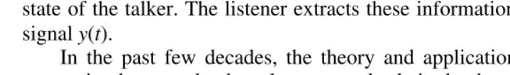
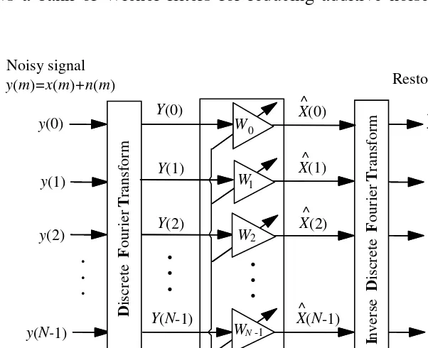
In many applications, for example at the receiver of a telecommunication system, there isno access to the instantaneous value of the contaminating noise, and only the noisy signal is available. In such cases the noise cannot be cancelled out, but it may be reduced, in an average sense, using the statistics of the signal and the noise process. Figure 1.4 shows a bank of Wiener filters for reducing additive noise when only the
. . . y(0)
y(1)
y(2)
y(N-1) Noisy signal
y(m)=x(m)+n(m)
x(0)
x(1)
x(2)
x(N-1)
^
^
^
^
I
nve
rs
e
D
is
cre
te
F
ou
ri
er
T
rans
fo
rm
.
.
.
Y(0)
Y(1)
Y(2)
Y(N-1)
D
is
cre
te
F
ou
ri
er
T
rans
fo
rm
X(0)
X(1)
X(2)
X(N-1)
^
^
^
^ WN-1
W0
W2
Signal and noise power spectra
Restored signal
Wiener filter estimator
W1
.
.
.
.
.
.
8 Introduction
noisy signal is available. The filter bank coefficients attenuate each noisy signal frequency in inverse proportion to the signal–to–noise ratio at that frequency. The Wiener filter bank coefficients, derived in Chapter 6, are calculated from estimates of the power spectra of the signal and the noise processes.
1.3.2 Blind Channel Equalisation
Channel equalisation is the recovery of a signal distorted in transmission through a communication channel with a non-flat magnitude or a non-linear phase response. When the channel response is unknown the process of signal recovery is called blind equalisation. Blind equalisation has a wide range of applications, for example in digital telecommunications for removal of inter-symbol interference due to non-ideal channel and multi-path propagation, in speech recognition for removal of the effects of the microphones and the communication channels, in correction of distorted images, analysis of seismic data, de-reverberation of acoustic gramophone recordings etc.
In practice, blind equalisation is feasible only if some useful statistics of the channel input are available. The success of a blind equalisation method depends on how much is known about the characteristics of the input signal and how useful this knowledge can be in the channel identification and equalisation process. Figure 1.5 illustrates the configuration of a decision-directed equaliser. This blind channel equaliser is composed of two distinct sections: an adaptive equaliser that removes a large part of the channel distortion, followed by a non-linear decision device for an improved estimate of the channel input. The output of the decision device is the final
Channel noise
n(m)
x(m) Channel distortion H(f)
f
y(m)
x(m)
^
Error signal
- +
Adaptation algorithm
+
f Equaliser
Blind decision-directedequaliser Hinv(f)
Decision device
+
Applications of Digital Signal Processing 9
estimate of the channel input, and it is used as the desired signal to direct the equaliser adaptation process. Blind equalisation is covered in detail in Chapter 15.
1.3.3 Signal Classification and Pattern Recognition
Signal classification is used in detection, pattern recognition and decision-making systems. For example, a simple binary-state classifier can act as the detector of the presence, or the absence, of a known waveform in noise. In signal classification, the aim is to design a minimum-error system for labelling a signal with one of a number of likely classes of signal.
To design a classifier; a set of models are trained for the classes of signals that are of interest in the application. The simplest form that the models can assume is a bank, or code book, of waveforms, each representing the prototype for one class of signals. A more complete model for each class of signals takes the form of a probability distribution function. In the classification phase, a signal is labelled with the nearest or the most likely class. For example, in communication of a binary bit stream over a band-pass channel, the binary phase–shift keying (BPSK) scheme signals the bit “1” using the waveform Acsinωct and the bit “0” using −Acsinωct. At the receiver, the decoder has the task of classifying and labelling the received noisy signal as a “1” or a “0”. Figure 1.6 illustrates a correlation receiver for a BPSK signalling scheme. The receiver has two correlators, each programmed with one of the two symbols representing the binary
Received noisy symbol
Correlator for symbol "1"
Correlator for symbol "0" Corel(1)
Corel(0)
"1
"
if
C
o
re
l(1
)
≥Co
re
l(
0)
"0
"
if
C
o
re
l(1
)
<
C
o
re
l(0
)
"1" Decision device
10 Introduction
states for the bit “1” and the bit “0”. The decoder correlates the unlabelled input signal with each of the two candidate symbols and selects the candidate that has a higher correlation with the input.
Figure 1.7 illustrates the use of a classifier in a limited–vocabulary, isolated-word speech recognition system. Assume there are V words in the vocabulary. For each word a model is trained, on many different examples of the spoken word, to capture the average characteristics and the statistical variations of the word. The classifier has access to a bank of V+1 models, one for each word in the vocabulary and an additional model for the silence periods. In the speech recognition phase, the task is to decode and label an
M ML
. . .
Speech signal
Feature sequence
Y
fY|M(Y|M1)
Word modelM2
likelihood ofM2
M
o
st
li
kel
y
w
ord
selec
to
r
Feature extractor
Word model MV Word modelM1
fY|M(Y|M2)
fY|M(Y|MV)
likelihood ofM1
likelihood ofMv
Silence modelMsil
fY|M(Y|Msil)
likelihood ofMsil
Applications of Digital Signal Processing 11
acoustic speech feature sequence, representing an unlabelled spoken word, as one of the V likely words or silence. For each candidate word the classifier calculates a probability score and selects the word with the highest score.
1.3.4 Linear Prediction Modelling of Speech
Linear predictive models are widely used in speech processing applications such as low–bit–rate speech coding in cellular telephony, speech enhancement and speech recognition. Speech is generated by inhaling air into the lungs, and then exhaling it through the vibrating glottis cords and the vocal tract. The random, noise-like, air flow from the lungs is spectrally shaped and amplified by the vibrations of the glottal cords and the resonance of the vocal tract. The effect of the vibrations of the glottal cords and the vocal tract is to introduce a measure of correlation and predictability on the random variations of the air from the lungs. Figure 1.8 illustrates a model for speech production. The source models the lung and emits a random excitation signal which is filtered, first by a pitch filter model of the glottal cords and then by a model of the vocal tract.
The main source of correlation in speech is the vocal tract modelled by a linear predictor. A linear predictor forecasts the amplitude of the signal at time m, x(m) , using a linear combination of P previous samples
x(m−1),,x(m−P)
[ ]as
∑
=− = P
k
kx m k a
m x
1
) ( )
(
ˆ (1.3)
where ˆ x (m) is the prediction of the signal x(m) , and the vector ]
, , [ 1
T
P a
a
=
a is the coefficients vector of a predictor of order P. The
Excitation Speech
Random source
Glottal (pitch) model
P(z)
Vocal tract model
H(z) Pitch period
12 Introduction
prediction error e(m), i.e. the difference between the actual sample x(m) and its predicted value ˆ x (m) , is defined as
e(m)= x(m) − akx(m−k) k=1
P
∑
(1.4)The prediction error e(m) may also be interpreted as the random excitation or the so-called innovation content of x(m) . From Equation (1.4) a signal generated by a linear predictor can be synthesised as
x(m)= akx(m−k) + e(m) k=1
P
∑
(1.5)Equation (1.5) describes a speech synthesis model illustrated in Figure 1.9.
1.3.5 Digital Coding of Audio Signals
In digital audio, the memory required to record a signal, the bandwidth required for signal transmission and the signal–to–quantisation–noise ratio are all directly proportional to the number of bits per sample. The objective in the design of a coder is to achieve high fidelity with as few bits per sample as possible, at an affordable implementation cost. Audio signal coding schemes utilise the statistical structures of the signal, and a model of the signal generation, together with information on the psychoacoustics and the masking effects of hearing. In general, there are two main categories of audio coders: model-based coders, used for low–bit–rate speech coding in
z–1 . . . z–1 z–1 u(m)
x(m-1) x(m-2)
x(m–P)
a a2 a1
x(m)
G e(m)
P
Applications of Digital Signal Processing 13
applications such as cellular telephony; and transform-based coders used in high–quality coding of speech and digital hi-fi audio.
Figure 1.10 shows a simplified block diagram configuration of a speech coder–synthesiser of the type used in digital cellular telephone. The speech signal is modelled as the output of a filter excited by a random signal. The random excitation models the air exhaled through the lung, and the filter models the vibrations of the glottal cords and the vocal tract. At the transmitter, speech is segmented into blocks of about 30 ms long during which speech parameters can be assumed to be stationary. Each block of speech samples is analysed to extract and transmit a set of excitation and filter parameters that can be used to synthesis the speech. At the receiver, the model parameters and the excitation are used to reconstruct the speech.
A transform-based coder is shown in Figure 1.11. The aim of transformation is to convert the signal into a form where it lends itself to a more convenient and useful interpretation and manipulation. In Figure 1.11 the input signal is transformed to the frequency domain using a filter bank, or a discrete Fourier transform, or a discrete cosine transform. Three main advantages of coding a signal in the frequency domain are:
(a) The frequency spectrum of a signal has a relatively well–defined structure, for example most of the signal power is usually concentrated in the lower regions of the spectrum.
Synthesiser coefficients
Excitation e(m)
Speech x(m) quantiser Scalar
Vector quantiser Model-based
speech analysis
(a) Source coder
(b) Source decoder
Pitch and vocal-tract coefficients
Excitation address
Excitation
codebook Pitch filter Vocal-tract filter
Reconstructed speech
Pitch coefficients Vocal-tract coefficients Excitation
address
14 Introduction
(b) A relatively low–amplitude frequency would be masked in the near vicinity of a large–amplitude frequency and can therefore be coarsely encoded without any audible degradation.
(c) The frequency samples are orthogonal and can be coded independently with different precisions.
The number of bits assigned to each frequency of a signal is a variable that reflects the contribution of that frequency to the reproduction of a perceptually high quality signal. In an adaptive coder, the allocation of bits to different frequencies is made to vary with the time variations of the power spectrum of the signal.
1.3.6 Detection of Signals in Noise
In the detection of signals in noise, the aim is to determine if the observation consists of noise alone, or if it contains a signal. The noisy observation
y(m) can be modelled as
y(m)=b(m)x(m) + n(m) (1.6)
where x(m) is the signal to be detected, n(m) is the noise and b(m) is a binary-valued state indicator sequence such that b(m)=1 indicates the presence of the signal x(m) and b(m)=0 indicates that the signal is absent. If the signal x(m) has a known shape, then a correlator or a matched filter
. . .
x(0)
x(1)
x(2)
x(N-1)
. . .
X(0)
X(1)
X(2)
X(N-1)
. . .
. . .
X(0)
X(1)
X(2)
X(N-1)
Input signal Binary coded signal Reconstructed signal
x(0)
x(1)
x(2)
x(N-1) ^
^
^
^
^
^
^
^ n0 bps
n1 bps
n2 bps
nN-1 bps
Transform
T
Encoder Decoder
. . .
Inverse Transform
T
-1
Applications of Digital Signal Processing 15
can be used to detect the signal as shown in Figure 1.12. The impulse response h(m) of the matched filter for detection of a signal x(m) is the time-reversed version ofx(m) given by
1 0
) 1 ( )
(m =x N− −m ≤m≤N −
h (1.7)
where N is the length of x(m) . The output of the matched filter is given by
∑
− =−
= 1
0
) ( ) ( )
( N
m
m y k m h m
z (1.8)
The matched filter output is compared with a threshold and a binary decision is made as
≥
=
otherwise 0
threshold )
( if 1 ) (
ˆ m z m
b (1.9)
where ˆ b (m) is an estimate of the binary state indicator sequence b(m),and it may be erroneous in particular if the signal–to–noise ratio is low. Table1.1 lists four possible outcomes that together b(m) and its estimate ˆ b (m) can assume. The choice of the threshold level affects the sensitivity of the
Matched filter
h(m)= x(N –1–m)
y(m)=x(m)+n(m) z(m)
Threshold comparator
b(m) ^
Figure 1.12 Configuration of a matched filter followed by a threshold comparator for detection of signals in noise.
ˆ
b (m) b(m) Detector decision 0 0 Signal absent Correct 0 1 Signal absent (Missed) 1 0 Signal present (False alarm) 1 1 Signal present Correct
16 Introduction
detector. The higher the threshold, the less the likelihood that noise would be classified as signal, so the false alarm rate falls, but the probability of misclassification of signal as noise increases. The risk in choosing a threshold value θ can be expressed as
(
Threshold=θ)
=PFalseAlarm(θ)+
PMiss(θ)R
(1.10)The choice of the threshold reflects a trade-off between the misclassification rate PMiss(θ) and the false alarm rate PFalse Alarm(θ).
1.3.7 Directional Reception of Waves: Beam-forming
Beam-forming is the spatial processing of plane waves received by an array of sensors such that the waves incident at a particular spatial angle are passed through, whereas those arriving from other directions are attenuated. Beam-forming is used in radar and sonar signal processing (Figure 1.13) to steer the reception of signals towards a desired direction, and in speech processing for reducing the effects of ambient noise.
To explain the process of beam-forming consider a uniform linear array of sensors as illustrated in Figure 1.14. The term linear array implies that the array of sensors is spatially arranged in a straight line and with equal spacing d between the sensors. Consider a sinusoidal far–field plane wave with a frequency F0 propagating towards the sensors at an incidence angle
of θ as illustrated in Figure 1.14. The array of sensors samples the incoming
Applications of Digital Signal Processing 17
wave as it propagates in space. The time delay for the wave to travel a distance of d between two adjacent sensors is given by
τ = dsinθ
c (1.11)
where c is the speed of propagation of the wave in the medium. The phase difference corresponding to a delay of τ is given by
c d F T
θ π
τ π
ϕ 2 2 0 sin
0 =
= (1.12)
where T0 is the period of the sine wave. By inserting appropriate corrective
WN–1,P–1 WN–1,1
WN–1,0
+
θ
0
1
N-1 Array of sensors
Inci dent
pla ne
wa ve
Array of filters
Output
. . . .
. .
. . .
W2,P–1 W2,1
W2,0
+
. . .z –1
W1,P–1 W1,1
W1,0
+
. . .d
θ
d sinθ
z –1
z –1
z –1
z –1
z –1
18 Introduction
time delays in the path of the samples at each sensor, and then averaging the outputs of the sensors, the signals arriving from the direction θwill be time-aligned and coherently combined, whereas those arriving from other directions will suffer cancellations and attenuations. Figure 1.14 illustrates a beam-former as an array of digital filters arranged in space. The filter array acts as a two–dimensional space–time signal processing system. The space filtering allows the beam-former to be steered towards a desired direction, for example towards the direction along which the incoming signal has the maximum intensity. The phase of each filter controls the time delay, and can be adjusted to coherently combine the signals. The magnitude frequency response of each filter can be used to remove the out–of–band noise.
1.3.8 Dolby Noise Reduction
Dolby noise reduction systems work by boosting the energy and the signal to noise ratio of the high–frequency spectrum of audio signals. The energy of audio signals is mostly concentrated in the low–frequency part of the spectrum (below 2 kHz). The higher frequencies that convey quality and sensation have relatively low energy, and can be degraded even by a low amount of noise. For example when a signal is recorded on a magnetic tape, the tape “hiss” noise affects the quality of the recorded signal. On playback, the higher–frequency part of an audio signal recorded on a tape have smaller signal–to–noise ratio than the low–frequency parts. Therefore noise at high frequencies is more audible and less masked by the signal energy. Dolby noise reduction systems broadly work on the principle of emphasising and boosting the low energy of the high–frequency signal components prior to recording the signal. When a signal is recorded it is processed and encoded using a combination of a pre-emphasis filter and dynamic range compression. At playback, the signal is recovered using a decoder based on a combination of a de-emphasis filter and a decompression circuit. The encoder and decoder must be well matched and cancel out each other in order to avoid processing distortion.
Applications of Digital Signal Processing 19
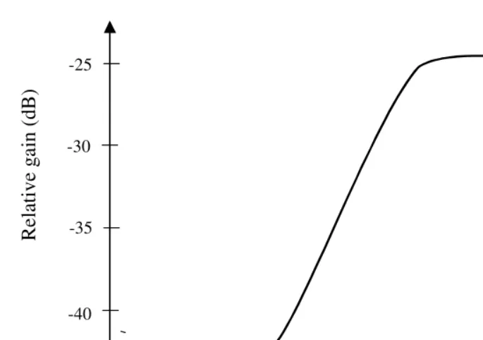
provides a maximum gain of 10 to 15 dB in each band if the signal level falls 45 dB below the maximum recording level. The Dolby B and Dolby C systems are designed for consumer audio systems, and use two bands instead of the four bands used in Dolby A. Dolby B provides a boost of up to 10 dB when the signal level is low (less than 45 dB than the maximum reference) and Dolby C provides a boost of up to 20 dB as illustrated in Figure1.15.
1.3.9 Radar Signal Processing: Doppler Frequency Shift
Figure 1.16 shows a simple diagram of a radar system that can be used to estimate the range and speed of an object such as a moving car or a flying aeroplane. A radar system consists of a transceiver (transmitter/receiver) that generates and transmits sinusoidal pulses at microwave frequencies. The signal travels with the speed of light and is reflected back from any object in its path. The analysis of the received echo provides such information as range, speed, and acceleration. The received signal has the form
0.1 1.0 1 0
-35
-45 -40 -30 -25
Re
lative ga
in
(
d
B
)
20 Introduction
]} / ) ( 2 [ cos{ ) ( )
(t A t 0 t r t c
x = ω − (1.13)
where A(t), the time-varying amplitude of the reflected wave, depends on the position and the characteristics of the target, r(t) is the time-varying distance of the object from the radar and c is the velocity of light. The time-varying distance of the object can be expanded in a Taylor series as
+ + +
+
= 2 3
0
! 3
1 !
2 1 )
(t r rt rt rt
r (1.14)
where r0 is the distance, r is the velocity, r is the acceleration etc.
Approximating r(t) with the first two terms of the Taylor series expansion we have
t r r t
r ≈ + 0
)
( (1.15)
Substituting Equation (1.15) in Equation (1.13) yields
] / 2
) / 2 cos[(
) ( )
(t A t 0 r 0 c t 0r0 c
x = ω − ω − ω (1.16)
Note that the frequency of reflected wave is shifted by an amount
c r d 2 ω0 /
ω = (1.17)
This shift in frequency is known as the Doppler frequency. If the object is moving towards the radar then the distance r(t) is decreasing with time, ris
negative, and an increase in the frequency is observed. Conversely if the
r=0.5Tc
cos(ω0t)
Cos{ω0[t-2r(t)
/c]}
Sampling and Analog–to–Digital Conversion 21
object is moving away from the radar then the distance r(t) is increasing, ris
positive, and a decrease in the frequency is observed. Thus the frequency analysis of the reflected signal can reveal information on the direction and speed of the object. The distance r0is given by
c T
r0 =0.5 × (1.18)
where T is the round-trip time for the signal to hit the object and arrive back at the radar and c is the velocity of light.
1.4 Sampling and Analog–to–Digital Conversion
A digital signal is a sequence of real–valued or complex–valued numbers, representing the fluctuations of an information bearing quantity with time, space or some other variable. The basic elementary discrete-time signal is the unit-sample signal δ(m)defined as
δ(m) = 1 m=0 0 m≠0
(1.19)
where m is the discrete time index. A digital signal x(m) can be expressed as the sum of a number of amplitude-scaled and time-shifted unit samples as
x(m) = x(k)δ(m−k) k=−∞
∞
∑
(1.20)Figure 1.17 illustrates a discrete-time signal. Many random processes, such as speech, music, radar and sonar generate signals that are continuous in
Discrete time
m
22 Introduction
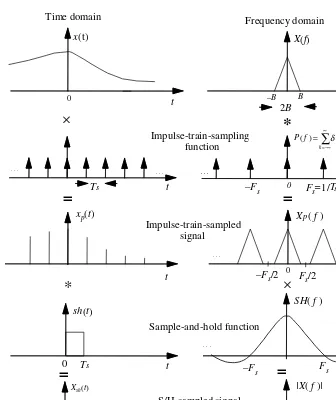
time and continuous in amplitude. Continuous signals are termed analog because their fluctuations with time are analogous to the variations of the signal source. For digital processing, analog signals are sampled, and each sample is converted into an n-bit digit. The digitisation process should be performed such that the original signal can be recovered from its digital version with no loss of information, and with as high a fidelity as is required in an application. Figure 1.18 illustrates a block diagram configuration of a digital signal processor with an analog input. The low-pass filter removes out–of–band signal frequencies above a pre-selected range. The sample– and–hold (S/H) unit periodically samples the signal to convert the continuous-time signal into a discrete-time signal.
The analog–to–digital converter (ADC) maps each continuous amplitude sample into an n-bit digit. After proc