DISCRIMINATION OF URBAN SETTLEMENT TYPES BASED ON SPACE-BORNE SAR
DATASETS AND A CONDITIONAL RANDOM FIELDS MODEL
T. Novack*, U. Stilla
Photogrammetry and Remote Sensing, TU München, 80333 Munich, Germany - (tessio.novack, stilla)@tum.de
Commission VI, WG VI/4
KEY WORDS: Urban structures types, Synthetic Aperture Radar, Conditional Random Fields
ABSTRACT:
In this work we focused on the classification of Urban Settlement Types (USTs) based on two datasets from the TerraSAR-X satellite acquired at ascending and descending look directions. These data sets comprise the intensity, amplitude and coherence images from the ascending and descending datasets. In accordance to most official UST maps, the urban blocks of our study site were considered as the elements to be classified. The considered USTs classes in this paper are: Vegetated Areas, Single-Family Houses and Commercial and Residential Buildings. Three different groups of image attributes were utilized, namely: Relative Areas, Histogram of Oriented Gradients and geometrical and contextual attributes extracted from the nodes of a Max-Tree Morphological Profile. These image attributes were submitted to three powerful soft multi-class classification algorithms. In this way, each classifier output a membership value to each of the classes. This membership values were then treated as the potentials of the unary factors of a Conditional Random Fields (CRFs) model. The pairwise factors of the CRFs model were parameterised with a Potts function. The reclassification performed with the CRFs model enabled a slight increase of the classification’s accuracy from 76% to 79% out of 1926 urban blocks.
* Corresponding author. This is useful to know for communication with the appropriate person in cases with more than one author.
1. INTRODUCTION 1.1 Urban Structure Types
Efficient urban planning and monitoring actions heavily rely on the spatial distribution of the city’s different settlements types. Waste production, traffic management, water and energy consumption are just a few socio-economic and environmental planning categories that should be tailored according to the spatial distribution of the city’s different types of settlements. In Germany, the term Urban Structure Types (USTs)
(Stadtstrukturtypen) was conceived in the nineties to categorize
these different urban settlements. Since then, this concept has been used as the main spatial indicator used in urban planning and monitoring actions in this country and others. Although there is no universally accepted definition of the term, USTs are usually understood as combining social and cultural aspects with the contextual and physical structure of the different settlements. More formally, USTs are characterized by: (1) the geometry, density and spatial configuration of buildings; (2) their social, cultural and economic usages (e.g. residential, commercial, industrial, amusement etc.) and (3) their environmental properties like the presence and type of vegetation and water bodies (Pauleit and Duhme (2000) and Heiden et al. (2012)).
1.2 Related Works and Our Contribution
Despite the tremendous potential of remote sensing data for rapidly providing accurate information on USTs, there has not been many works explicitly devoted to their automatic detection and classification based on remote sensing data. Most of these works have utilised multispectral (Banzhaf and Höfer, 2008; Wurm et al., 2009; Huck et al., 2011; Wade et al., 2014),
hyperspectral (Heldens, 2010; Heiden et al., 2012) imagery or simply some elevation data or vector dataset of the buildings (Steiniger et al., 2008; Yu et al., 2010; Wurm and Taubenboeck, 2010).
A common approach seems to be to extract first land cover objects and then, according to certain measures of their structure inside a spatial parcel (usually the urban blocks), estimate its UST. Huck et al. (2011) classified USTs at the block-level hierarchically applying thresholds on the relative area and density of land cover classes inside the blocks. Wade et al. (2014) also proposed the classification of USTs based on the topology of land cover objects extracted inside urban blocks. The topology is described by different measures of neighbourhood-graphs, which are then submitted to a random forest classifier. Heiden et al. (2012) used airborne hyperspectral and elevation data to map the USTs of Munich (Germany). They first perform land cover classification and correct it using elevation data, which is also used to derive urban volume indicators. Topographic maps and cadastral data on buildings in vector format have also been used for deriving the USTs of urban blocks. Steiniger et al. (2008) used cadastral vector data of the buildings from Zurich (Switzerland) and their morphological and contextual properties to distinguish USTs based on the results of different classifiers. They rely on the assumption that buildings from a same UST have similar shape and distances between each other. Hecht et al. (2013) extracted building footprints from topographic maps and classified them according to a considered building typology. Following, urban blocks are classified into USTs depending on the dominating building type.
Without ever mentioning the term USTs, different research groups have tried to distinguish types of urban settlements based on medium-resolution Synthetic Aperture Radar (SAR) ISPRS Annals of the Photogrammetry, Remote Sensing and Spatial Information Sciences, Volume II-3/W4, 2015
data. These works rely most of the times on textural attributes and simple backscattering measures (Weydahl, 2002; Dekker, 2003; Dell’Acqua and Gamba, 2006). Hoefner et al. (2009) in the other hand proposed jointly using high-resolution SAR and multispectral data to classify USTs. They suggest the use of a set of rules for USTs classification, which can be later improved based on textural features from SAR imagery. Nevertheless, they presented only very initial results.
From this brief overview, it is possible to notice that the classification of UST based solely on high-resolution SAR imagery has explicitly not been tried yet. Motivated by that, we investigate the feasibility of automatically classifying general USTs based on high-resolution space-borne SAR data from ascending and descending look directions. Since the information content of SAR data is heavily related to the geometrical properties of the surface objects, we assume such data can be used to attain this goal. Differently from any other research in this direction, we focus in this paper on the classification of USTs followed by their reclassification by a probabilistic graphical model, more specifically, a Conditional Random Fields (CRFs) model (Lafferty et al. 2001). The consideration of the contextual relations between the USTs classes of neighbouring urban blocks was expected to increase the classification accuracy.
2. METHODS 2.1 Semantic Grouping of UST Classes
Based solely on remote sensing data, it is very hard to distinguish two UST classes that do not differ on their physical aspects but only on their land use. Also, some UST classes are very specific on their land use and physical structure, what makes them rarely found on the urban area. Hence, we decided to exclude from our analysis these few rare and very specific classes and to group the remaining ones into three semantically broad USTs, namely: Parks and Vegetated Areas, Single-Family Houses and Commercial and Residential Buildings.
2.2 Data Preparation and Image Partitioning
For the realization of our experiments, two interferometric datasets from the TerraSAR-X satellite from the city of Munich (Germany) were used, being one of these datasets acquired at ascending look direction and another at descending look direction (Table 1). All images were obtained in High-Resolution Spotlight mode, which yields a pixel spacing of approximately 1,1 m. Each dataset comprises the intensity and amplitude images from the master acquisition, as well as the computed coherence image. All images were kept in their original acquisition orientation, so that no information distortion would be caused by re-projecting them.
The first step of our processing chain was the partitioning of the images into segments. This was achieved by overlaying the vector data from the streets, water bodies and railroad tracks onto the images. In this way, the obtained segments coincided exactly with the borders of the vector objects. Since urban constructing blocks are usually delimited by the street and railroad networks, the borders of our segments coincide exactly with those from the urban blocks of the study area. This superposition of the vector and image data was possible because both are geo-referenced and it only demanded the turning of the vector data to the orientation of the images.
Look
Descending 09.05.2011 120.16 27.32 m 20.05.2011
Table 1. Acquisition parameters of the TerraSAR-X imagery.
2.3 Image Attributes
It is not easy to discover expressive image attributes for the classification of USTs. This task becomes even more difficult when deriving these attributes from SAR images. Ideally, the attributes must express the contextual, geometrical and spectral structure of the whole block in order to be informative
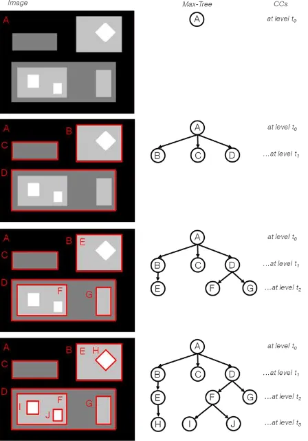
Figure 1. Example of a MT-MP from a synthetic image. The CCs are groups of neighbouring pixels whose values are above
the level’s threshold (represented in red at the images on the right). On the left side the corresponding hierarchically
structured tree is depicted.
Relative Areas concern the proportion of pixels inside an urban block whose values are below or above a certain threshold. Although simple, this group of attributes can be very powerful, especially when combined with other attributes in a classification scheme. The high-threshold and low-threshold ISPRS Annals of the Photogrammetry, Remote Sensing and Spatial Information Sciences, Volume II-3/W4, 2015
were defined by calculating ten percentiles of each image and selecting the second and the eighth percentile values as the high- and low-thresholds respectively. A third threshold value was calculated using the Otsu’s method, which calculates an optimal threshold by maximizing the variance between two classes of pixels (separated by the threshold). Equivalently, this threshold minimizes the intra-class variance. For this paper we calculated (1) the proportion of pixels from the amplitude and intensity images above the high-threshold; (2) the proportion of pixels from the amplitude and intensity images below the low- threshold and (3) the proportion of pixels from the coherence images above and below the Otsu threshold. These calculations were done on the images from the ascending and descending datasets, adding to a total of twelve attributes. In this way, we were able to extract for each block the proportions of (1) strong backscattering objects; (2) shadowed or occluded areas and (3) vegetated areas, since vegetation and water have low coherence values whereas man-made structures have high coherence values.
HOGs are powerful image descriptors regarding computer vision applications (Dalal and Triggs, 2005). Their expressiveness as attributes for classifying remote sensing imagery has not yet been extensively exploited. HOGs can describe an urban block by the magnitude and direction of the gradients and then accumulating a histogram over it. The gradients are calculated over a certain number of squared cells with a certain size.
The third type of image attributes used in this paper required the creation of a MT-MP by the application of several thresholds on the images with increasing values. At the application of each threshold a binary image is produced, where pixels receive value 1 in case they have values above the threshold and 0 otherwise. Pixels spatially grouped whose values are above the threshold are called connected components (CC). As the application of the subsequent higher thresholds image. From these regions, several geometrical, positional and contextual attributes can be calculated. In this work, the considered geometrical attributes were area, rectangular fit and
length-width division. We also considered the position of the
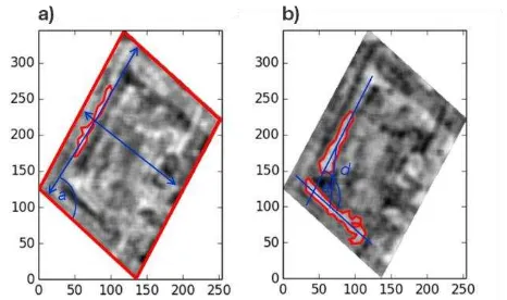
CC’s region in relation to the borders of the urban block and in relation to other CCs whose geometrical attributes are in accordance to a CC considered as a building hypothesis. In other words, we check for each CC, based on its geometrical attributes, whether it can be considered to be a building or a house or none of the two. In case, it can be considered to be a building, we calculated its distance and angle difference to the borders of the block (Figure 2a). As mentioned, each pair of CCs understood as buildings had their relative angle and distance calculated (Figure 2b)
2.4 Classification Attributes and Strategy
In this work we created one MT-MP for each block and for the intensity and amplitude images of each of the two SAR datasets, making a total of four MT-MPs four each block. After creating each three, we counted (1) the number of CCs considered as buildings, (2) the number of CCs considered as
house, (3) the number of buildings parallel to one of the borders of the block and close enough to it, (4) the number of CCs pairs that were considered as buildings and that were orthogonal to each other and (5) the number of CCs pairs that were considered as buildings and that were orthogonal to each other. These image attributes are referred from now on as morphological attributes (MAs).
Figure 2. Distance of a CC to the borders of the block (a) and relative distance and orientation between two CCs considered
as buildings.
The HOGs features were calculated separately for each block and for the intensity, amplitude and coherence images of each of the looking-directions, making a total of six histograms for each block. Each histogram was accumulated for nine directions from nine different cells. The size of the cells varied according to the size of the urban block. The magnitudes of the gradients at each direction were also considered as attributes, together with the highest gradient magnitude of each histogram and its corresponding angle. This added up to 66 attributes calculated for each block. We refer to this group of attributes from now on as HOGs Descriptors.
Each group of attributes was submitted separately to three powerful soft classifiers of our choice, namely: Random Forest (Breiman, 2001), Logistic Regression and Nearest-Neighbours. These classifiers are soft because they deliver a membership value (between 0 and 1) to each class for each urban block. Figure 3 shows how the classification strategy was organised. Since we have three groups of attributes, three classifiers and three classes, each block is associated to twenty-seven membership values, i.e. nine to each class. We aggregated them by calculating their arithmetic mean. Each block was in this way associated to one membership value to each of the three classes. A first classification was then performed by selecting for each block the class with the highest membership value.
Figure 3. Ensemble of soft classifiers used for our experiments. Each group of attributes was submitted to each of the classifiers adding to a total of nine output membership values for each
class and for each block.
2.5 Construction of the CRFs graph
A CRFs model possesses two types of factors: the ones composed of at least one observed variable and one not-observed variable and the ones composed only of not-not-observed variables. In our case, the not-observed variables are the unknown USTs class of each block. The observed variables are the membership of each block to each of the three USTs classes we consider in this study. Their computation is explained on section 2.4. Our simple CRFs model has two different types of factors with exactly two variables each. One is composed of one observed variable and one not-observed variable. We call this factors unary factors. Each urban block has exactly one unary factor. The other type of factor present in our model is the one involving the not-observed variable of a block and the not-observed variable of one of its neighbours. Each block has the same amount of this factor as the number of neighbours it has. We call these factors the pairwise factors. The parameterization of the unary factors is straightforward: the parameters are exactly their membership values to the classes. The parameters of the pairwise factors were defined using a so-called Potts function:
The Potts pairwise parameterization defines that preferably the classes of two neighbouring blocks should be the same. This assignment receives potential 10. The potential to the case were the classes of two neighbouring blocks differ is 2.
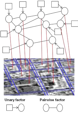
In order to define whether two blocks are neighbours, a distance criterion was applied. The centroid of each block was extracted along with their image coordinates. Following, the distance matrix containing all blocks was generated. Finally, two blocks are considered to be neighbours if the distance to each other is below the threshold of 300 meters. Figure 4 enables an intuitive understanding of our CRFs graph. The squares are the variable containing the membership values to the UST classes for each block. The circles represent the unknown UST class of the block. Each block is associated to one unary factor on the graph and to the amount of pairwise factors as its number of neighbours.
Once we have created and parameterized the CRFs model, the next step was to run inference over it in order to estimate the most probable classification of the scene. We used the standard and powerful algorithm for approximate inference named Loopy Belief Propagation (Kschischang et al., 2001) for this task. This algorithm together with other functions for the creation of probabilistic graphical models is available in the OpenGM library (Andres and Kappes, 2012).
3. RESULTS AND DISCUSSION
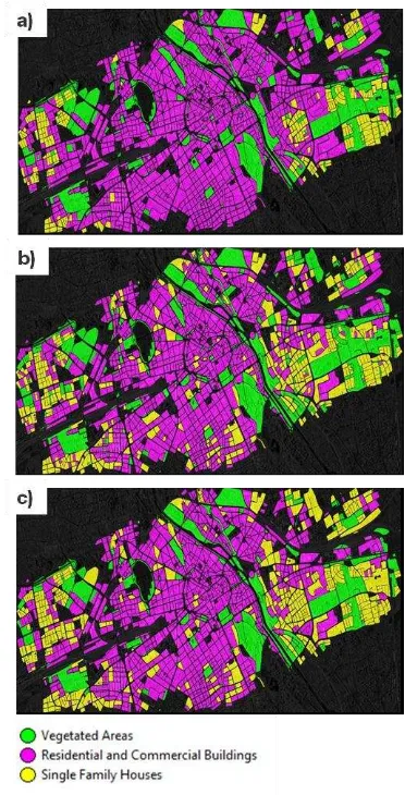
In this section we present and discuss the classification and re-classification results and discuss them. Figure 5 shows three classifications. The UST ground-truth map is shown on Figure 5a. It was produced by semantically grouping the UST classes (section 2.1) from the official UST map from Munich. This map was kindly provided to us by the prefecture of this city and it considers the urban blocks as the elementary mapping units, which enabled a one-to-one comparison between the map and the classifications.
The classification achieved with the three groups of image attributes submitted to the classification strategy presented on
section 2.4 is shown in Figure 5b. This classification has an overall accuracy of 76%. Its confusion matrix along with its per-class accuracies are shown in Table 2.
Figure 4. Construction of the CRFs model. Squares represent the observed variables and the circles represent the unknown UST class of the blocks. A pairwise factor is created between two blocks if they are considered to be neighbours by a distance
criterion.
With the application of the CRFs model, an increase of only 3% was achieved. On the other hand, one notices by looking at Figure 5 that the CRFs classification is slightly smoother and in little more accordance with the distribution of the classes in the ground-truth map. In the other hand, as shown in Figure 6a, some mistaken class changes occurred with the reclassification. Figure 6b show example of successful class changes. They outnumber the incorrect changes, but the overall improvement of the classification is less than expected. Nevertheless, the fine tuning of the Potts function parameters and the distance criterion for neighbourhood definition may improve the results significantly. Because of that we will focus on the development of rules to regulate the pairwise interaction of neighbouring blocks based not only on their distance, but also on their geometrical similarities. Also, the potential of each class combination on the pairwise factors can be further tuned based on their a priori probabilities extracted from the sample set used for training the soft classifiers.
4. DISCUSSION
This paper shows our first efforts to classify general UST classes based on simple statistical and geometrical image attributes. Despite the existence of a few papers that propose the classification of UST based on urban blocks and other remote sensing datasets, none of them evaluate the possibility of using solely (In)SAR data. This research has the additional novelty hence of also including a second InSAR dataset into play. Despite the fact that we did not consider the elevation data possible to be obtained by interferometric means, we showed a simple way of considering the distribution of objects inside the urban blocks and using this information as an attribute. This, together with the extraction of vegetation and man-made ISPRS Annals of the Photogrammetry, Remote Sensing and Spatial Information Sciences, Volume II-3/W4, 2015
structures from the coherence, intensity and amplitude images, enabled the classification of general USTs with good accuracy. The main contribution of this paper is though the fact that the context between neighbouring urban blocks is considered in a probability-based reclassification of the image based on a simple but elegant CRFs model. We expect to transmit our acquired motivation to other researchers in the field for putting efforts in the direction of considering broader contexts in the block-based urban land-use and UST classification.
Figure 5. Ground-truth UST map (a), classification obtained with the ensemble of classifiers (b) and the reclassification
obtained by the application of the CRFs model (c).
Confusion Matrix
VA SFH CRB Sum
VA 240 0 12 252
SFH 21 279 275 575
CRB 5 16 951 972
Unclassified 108 4 15 127
Sum 374 299 1253
Accuracy Indexes (Classes)
Producer 0.64 0.93 0.76
User 0.95 0.48 0.97
Kappa 0.58 0.90 0.51
Totals
Overall Accuracy 76%
Kappa 0.61
Table 2. Confusion matrix and class accuracy indexes of the UST classification. The name of the classes is shown
abbreviated – Vegetated Areas (VA), Single Family Houses (SFH) and Commercial and Residential Buildings (CRB).
Figure 6. Examples of erroneous (a) and successful (b) class changes performed by the CRFs-based reclassification step.
ACKNOWLEDGEMENT
We acknowledge the financial help given by the Deutscher Akademischer Austausch Dienst (DAAD) during the time in which this paper was written, as well as the Referat fuer Gesundheit und Umwelt der Stadt Muenchen for providing us with the up-to-date official USTs map.
REFERENCES
Andres, B. T. and Kappes, J. H. 2012. OpenGM: A C++ library for discrete graphical models. ArXiv e-prints.
Banzhaf, E. and Höfer, R., 2008. Monitoring Urban Structure Types as Spatial Indicators With CIR Aerial Photographs for a More Effective Urban Environmental Management. Journal of Selected Topics in Applied Earth Observations and Remote
Sensing, 1(2), pp. 129-138.
Breiman, L. 2001. Random Forests, Machine Learning, 45, pp. 5-32.
Dalal, N. and Triggs, B., 2005. Histograms of oriented gradients for human detection. In: IEEE Computer Society Conference on ISPRS Annals of the Photogrammetry, Remote Sensing and Spatial Information Sciences, Volume II-3/W4, 2015
Computer Vision and Pattern Recognition, Vol. I, pp. 886-893. Dekker, R.J., 2003. Texture analysis and classification of ERS SAR images for map updating of urban areas in the Netherlands. IEEE Transactions on Geoscience and Remote
Sensing, 41, pp. 1950-1958.
Dell'Acqua F. and Gamba P. 2006. Discriminating urban environments using multiscale texture and multiple SAR images. International Journal of Remote Sensing, 27(18), pp. 3797-3812.
Hecht, R., Herold, H., Meinel, G. and Buchroithner, M. 2013. Automatic derivation of urban structure types from topographic maps by means of image analysis and machine learning. In: Buchroithner, M. et al. (Eds.): 26th International Cartographic
Conference.
Heiden, U., Heldens, W., Roessner, S., Segll, K., Esch, T. and Mueller, A., 2012. Urban structure type characterization using hyperspectral remote sensing and height information.
Landscape and Urban Planning, 105, pp.361-375.
Heldens, W., 2010. Use of airborne hyperspectral data and height information to support urban micro climate characterisation. Bayerischen Julius-Maximilians-Universitaet Wuerzburg, PhD Dissertation, Germany.
Hoefner, R., Banzhaf, E. and Ebert, A. (2009) Delineating urban structure types (UST) in a heterogeneous urban agglomeration with VHR and TerraSAR-X data. 2009 Urban Remote Sensing Joint Event.
Huck, A., Hese, S. and Banzhaf, E., 2011. Delineating parameters for object-based urban structure mapping in Santiago de Chile using Quickbird data. In: International Archives of the Photogrammetry, Remote Sensing and Spatial
Information Sciences, Hannover, Germany, Vol.
XXXVIII-4/W19.
Kschischang, F., Frey, B. and Loeliger, H. A. 2001. Factor-graphs and the sum-product algorithm. IEEE Transactions on
Information Theory, 47, pp. 498-519.
Lafferty, J., MacCallum, A. and Pereira, F. 2001. Conditional random fields: Probabilistic models for segmenting and labeling sequence data. In proc. 18th International Conference on machine Learning (ICML).
Munich, 2014. Referat fuer Gesundheit und Umwelt der Stadt Muenchen.http://www.muenchen.de/rathaus/Stadtverwaltung/R eferat-fuer-Gesundheit-und-Umwelt.html (30 Jul. 2014).
Novack, T. and Stilla, U. (2014) Discriminative learning of Conditional Random Fields applied for the classification of urban settlements types. In: Wissenschaftlich-Technische
Jahrestagung der DGPF, Hamburg, Germany, Vol. XXXIV.
Pauleit, S. and Duhme, F., 2012. Assessing the environmental performance of land cover types for urban planning. Landscape
and Urban Planning, 52, pp.1-20.
Steiniger, S., Lange, T., Burghardt, D. and Weibel, R., 2008. An approach for the classification of urban buildings structures based on discriminant analysis techniques. Transactions in GIS, 12(1), pp. 31-59.
Walde, I., Hese, S., Berger, C. and Schmullius, C., 2014. From land cover graphs to urban structure types. International
Journal of Geographical Information Science, 28(3), pp.
584-609.
Weydahl, D.J., 2002. Backscatter changes of urban features using multiple incidence angle RADARSAT images. Canadian
Journal of Remote Sensing, 28(6), pp.782-793.
Wurm, M., Taubenböck, H., Roth, A. and Dech, S., 2009. Urban structuring using multisensoral remote sensing data – by the examples of german cities – Cologne and Dresden. In:
Urban Remote Sensing Joint Event, Shanghai, China.
Wurm, M. and Taubenböck, H. 2010. Fernerkundung als Grundlage zur Identifikation von Stadtstrukturtypen. In:
Fernerkundung im urbanen Raum, Darmstadt, Germany, pp.
94–103.
Yu, B., Liu, H., Wu, J., Hu, Y. and Zhang, L., 2010. Automated derivation of urban building density information using airborne LiDAR data and object-based method. Landscape and Urban
Planning, 98, pp. 210-219.