Estimating daytime latent heat flux and evapotranspiration in Jamaica
D. Amarakoon
∗, A. Chen, P. McLean
Department of Physics, University of the West Indies, Kingston 7, West Indies, Jamaica Received 20 July 1999; received in revised form 6 January 2000; accepted 14 January 2000
Abstract
The suitability of the two-parameter scheme of De Bruin and Holtslag (1982) to estimate daytime latent heat flux and evapotranspiration in Jamaica was examined using meteorological data collected over fields of short grass. The study covered three different periods, January to February of 1994, January to February of 1990, and August to September of 1989. The fields were irrigated regularly (three times a week) to provide enough water to evaporate. The daytime (07:00–18:00 hours) 20 min and hourly latent heat flux values, average evaporation for the earlier mentioned three periods and evaporation on individual days were estimated using De Bruin and Holtslag scheme for two situations. One was with the parameterα′=0.95 andβ=20 W m−2and the other was withα′=1.05 and
β=20 W m−2. The analysis of the latent heat flux and evaporation led
to the following results. (i) The values of latent heat flux and evaporation estimated usingα′=0.95 andβ=20 W m−2compare
well with the corresponding measured values for time steps of the order of 20 min to several days. (ii) The level of agreement between estimated and measured hourly values of latent heat flux seen in our work was very close to that reported in the study of De Bruin and Holtslag, implying the consistency of the skill of that scheme at higher average latent heat flux levels in Jamaica. (iii) The choice of 1.05 forα′applies better for our data. These results indicate that the scheme of De Bruin and Holtslag withα′=0.95 and
β=20 W m−2can satisfactorily be used to estimate daytime latent heat flux and evaporation from
well watered grass surfaces in regions having environmental conditions similar to those encountered in Jamaica, but appears better withα′=1.05. © 2000 Elsevier Science B.V. All rights reserved.
Keywords:Grass; Bowen ratio; Latent heat flux; Evaporation; Radiation; Priestly–Taylor parameter
1. Introduction
Estimation of surface latent heat flux and hence ac-tual evaporation (evapotranspiration) from surfaces is important for purposes such as regional water bal-ance studies, field irrigation practice, description of the atmospheric boundary layer including stability, and weather forecasting. Many schemes are available to accomplish the estimation (Brutsaert, 1982). However, little work has been done on evaporation in the tropics and all the schemes available have been developed in
∗Corresponding author. Fax:+1-876-977-1595.
E-mail address:[email protected] (D. Amarakoon)
temperate climates. The lack of information on evap-oration in the tropics leads to situations where avail-able schemes have to be used to estimate evaporation without any prior knowledge of their applicability to tropical environmental conditions. This can cause er-rors in the estimates.
Three schemes (Penman, 1948; Priestley and Tay-lor, 1972; De Bruin and Holtslag, 1982) need to be mentioned. The schemes (Penman, 1948; Priestley and Taylor, 1972) are important as they are widely used in hydrology because of their sound analytical basis, and also they have resulted in other schemes (e.g. Brutsaert and Stricker, 1979; De Bruin and Holtslag, 1982) that are of practical value. The scheme of De
Bruin and Holtslag (1982) is a simple empirical mod-ification of Priestley and Taylor (1972) scheme, and it appears useful in estimating surface latent heat flux from surfaces with short crops when the surface is supplied with enough water to evaporate. The prac-tical advantage of this scheme is the fact that only a few measurable input parameters are required to es-timate latent heat flux apart from the two empirical parameters α′ and β. The results of De Bruin and
Holtslag (1982) have shown that the scheme has the same skill as Penman–Monteith approach (Monteith, 1965; Brutsaert, 1982). Penman–Monteih approach (Monteith, 1965; Brutsaert, 1982) is a more complete scheme, but requires a relatively large number of input parameters.
The objective of our study was to examine the ap-plicability of De Bruin and Holtslag (1982) scheme for estimating latent heat flux and evaporation in Ja-maica, which has a tropical climate. The scheme was developed in the Netherlands, which has a temperate climate and appear to have the potential for practical applications. If its applicability can be verified under tropical environmental conditions, it may be a useful tool, especially in agricultural meteorology, for esti-mating latent heat flux and hence evaporation from surfaces covered with short vegetation and irrigated regularly. For testing De Bruin and Holtslag (1982) scheme, we estimated the quantities stated below using that scheme and the data collected over fields with grass during the periods January to February of 1994, January to February of 1990 and August to September of 1989. The quantities estimated were daytime (07:00–18:00 hours) values of (i) 20 min and hourly latent heat flux, (ii) average evaporation for the three periods of data collection and (iii) evaporation on individual days. The estimated values were then compared with corresponding measured values using linear regression analysis and calculating percentage deviations where appropriate.
2. Consideration of schemes
The Penman scheme (Penman, 1948) which was originally intended for evaporation from an open-water surface, but shows general applicability to any wet surface (Brutsaert, 1982), can be cast in the form (including the heat flux into the surface):
E=
whereEis the evaporation in mm during the time in-tervalŴin seconds,e* andeare the saturation vapor pressure at air temperature θ and vapor pressure in mb, respectively,1the slope of thee* versus air tem-perature curve atθ,Rnthe net radiation in W m−2,G
the heat flux into the surface in W m−2,λ the latent
heat of vaporization andγthe psychrometric constant which is equal tocpp/(0.622). In the definition of γ, cp is the specific heat capacity of dry air at constant
pressure,p is the atmospheric pressure and 0.622 is the ratio of the molecular weight of water vapor to that of dry air. In Eq. (1) the functionf(u) is a func-tion of the wind speedu and the product f(u)(e*−e) is in mm day−1. The form off(u) originally proposed
by Penman (1948) is the following.
f (u)=0.26(1+0.54u) (2)
whereuis the mean wind speed in m s−1at 2 m above
the surface. The expression corresponding to Eq. (1) that represents the latent heat flux,lin W m−2, can be
The scheme of Priestley and Taylor (1972) is the best-known simplification of Penman (1948) scheme and is based on the concept of equilibrium evapora-tion (Slatyer and McIlroy, 1961) from moist surfaces. Slatyer and McIlroy (1961) had presented the idea that over a very large homogeneous and thoroughly moist surface under well established steady conditions
etends toe*. A consequence of this is the vanishing of the second term containing (e*−e) from Eq. (1) and hence the first term in Eq. (1) may be considered to represent a lower limit to evaporation from moist surfaces which the authors referred to as the equilib-rium evaporation. In our work, equilibequilib-rium evapora-tion is denoted by Eeq and the corresponding
equi-librium latent heat flux which is the first term on the right hand side of Eq. (3) is denoted byleq. Priestley
and Taylor (1972) treated the equilibrium evaporation as the basis for an empirical relationship for evapora-tion from a wet surface under condievapora-tions of minimal advection. After analyzing data over ocean and satu-rated land surfaces they presented a scheme for wet surface evaporation, which is of the form
E=αEeq (4)
where the parameter α in Eq. (4) is known as the Priestley–Taylor parameter or coefficient. For large saturated land and advection-free water surfaces, Priestley and Taylor (1972) concluded that the best estimate forαis 1.26. As mentioned in the literature (Brutsaert, 1982; Cargo and Brutsaert, 1992) there is enough experimental evidence to support the va-lidity of a value around 1.26 for α. Eichinger et al. (1996) have derived an analytical expression for α
and their results have shown good agreement with the value 1.26. The equation for the latent heat fluxl
corresponding to Eq. (4) is
l=αleq (5)
The scheme of De Bruin and Holtslag (1982) can be presented in the form
whereα′ andβ are empirical constants and the first
term on the right-hand side is the same asα′l
eq.
Ac-cording to the energy balance equation for the earth’s
surface,Rn,G,land the sensible heat fluxHcan be
linked by the equation,
Rn=l+H+G (7)
Combining Eqs. (6) and (7), the sensible heat fluxH
can be given by
De Bruin and Holtslag (1982) have performed mea-surements over a 100 m×100 m field covered with short grass of about 8 cm in height. They have ana-lyzed data for two periods. During one period, which they call the normal period, the ground had been wet-ter than the other period to which they refer as the dry period. For the normal period, the analysis of hourly latent heat flux data has shown thatα′
can be assigned the value 0.95 and theβvalue 20 W m−2. For the dry
period, the values are 0.65 and 20 W m−2, respectively.
The results have shown that the hourly values ofl es-timated using Eq. (6) and the aboveα′ andβ values
compare well with experimentally determinedlvalues and the values calculated using the Penman–Monteith approach (Monteith, 1965; Brutsaert, 1982) which is a more complete scheme. The values ofHestimated using Eq. (8) have also shown reasonably good agree-ment (correlation coefficient of 0.92 and a root mean square error of 38% of average H) with experimen-tally determinedHvalues. Furthermore, their results have indicated that daily mean ofα(Priestley–Taylor coefficient) is about 10% greater than its hourly value during daytime, and thatα=1.26 yields good results for daily values of latent heat flux.
3. Site description and environmental conditions
The experimental sites were located at Mona and St. Catherine in Jamaica, West Indies. The latitude, longitude and altitude respectively for the stations are as follows: 17◦
W and 150 m for St. Catherine. The distance from Mona to St. Catherine is 35 km. The site at Mona was situated on an open rectangular lot of extent 120 m×80 m. The other site was located at
Table 1
The number of data collection days and the daytime (07:00–18:00 hours) average environmental conditions under which the experiments were performed during August to September of 1989, January to February of 1990 and January to February of 1994
Parametera August–September 1989 January–February 1990 January–February 1994
N 26 31 32
Rs (W m−2) 170.0–890.0 90.0–750.0 73.5–629.6
Rn(W m−2) 74.2–564.2 37.1–473.0 6.7–394.0
θ (◦C) 25.3–32.1 20.7–30.0 22.9–28.3
u(m s−1) 0.6–4.4 0.5–5.2 0.8–3.2
δe(mb) 2.08–15.6 6.9–18.9 7.3–15.6
Average RH (%) 81 63 79
L(m) −0.014 to−275 (0.004) −4 to−348 (2.7) −6 to –151 (0.04)
aDefinitions of the parametersR
s,Rn,θ, u, and RH are the same as in Table 2.N=number of data collection days andδe=vapor pressure deficit. The relative humidity shown is the ratio, vapor pressure measured at 1.5 m to saturation vapor pressure calculated using the result of Lowe (1977). The measured average relative humidity in 1994 was 73%.Lis the Monin–Obukhov length estimated by the method outlined in Appendix A. The positive values ofLwithin parentheses are for stable situations in the morning at 07:00 hours or in the late afternoon at 17:00 hours. 75% of theLvalues were in the range−150<L<0 m. The values of all the quantities given are hourly average values, exceptN. Hourly average values refer to averages for each hour between 07:00 and 18:00 hours.
upwind and 30 m downwind, followed by an embank-ment about 10 m high. The wind was primarily from the south. The surfaces at both sites were covered with grass of Bahamian variety of average height 10 cm and were irrigated regularly, three times a week, to ensure that there was enough water to evaporate. The average of the ratio, l(measured)/leq, was 1.17 based
on hourly values of the fluxes. The top soil surface at both sites was mainly loam. The data collection period at Mona was January to February of 1994, and the periods at St. Catherine were August to September of 1989 and January to February of 1990. The daytime environmental conditions during the three periods and the number of data collection days are given in Table 1. The atmosphere was predominantly
unsta-Table 2
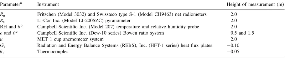
Parameters measured, instruments used and the height of measurements in this study, during the periods: August to September of 1989, January to February of 1990 and January to February of 1994
Parametera Instrument Height of measurement (m)
Rn Fritschen (Model 3032) and Swissteco type S-1 (Model CH9463) net radiometers 2.0
Rs Li-Cor Inc. (Model LI-200SZC) pyranometer 2.0
RH andθb Campbell Scientific Inc. (Model 207) temperature and relative humidity probe 2.0
eandθc Campbell Scientific Inc. (Dew-10 series) Bowen ratio system 0.5 and 1.5
u MET 1 cup anemometer system 2.0
Gs Radiation and Energy Balance Systems (REBS), Inc. (HFT-1 series) heat flux plates −0.10
θs Thermocouples −0.05
aR
n=net radiation, Rs=global short-wave radiation, RH=relative humidity, θ=air temperature, e=vapor pressure, u=wind speed, Gs=soil heat flux at 0.10 m below the surface,θs=soil temperature at 0.05 m below the surface.
bRH measured only in January–February of 1994.
cBowen ratio system provided measurements ofeandθ at 0.5 m and 1.5 m.
ble, as indicated by the estimated values of Monin– Obukhov length L. A few early morning and late afternoon L values depicted stable (L>0) or neutral (|L|>150 m) conditions. The method of estimation of
Lis given in Appendix A. The atmospheric instability observed in this work agrees with the other studies (Hsu, 1982; Chen et al., 1990) on tropical atmospheric instability.
4. Measurements and methods
in Table 1. The data were stored on-site as 20 min av-erages in a datalogger (Campbell Scientific Inc. 21X micrologger) and downloaded to a computer for anal-ysis. The surface fluxesl,HandGwere determined using the procedures outlined in Sections 4.1, 4.2 and 4.3 later. The values ofl(andE),HandGdetermined in this manner are referred to as the measured values of these quantities.
4.1. Determination of l and H
Bowen ratio energy balance method was used to determine the latent heat flux (l) and the sensible heat flux (H). Bowen ratio,Bo, is equal toH/l(Brutsaert,
1982). Combination of this result with Eq. (7) provides the expression forlgiven in Eq. (9).
l= (Rn−G)
(1+Bo) (9)
The values oflcan be calculated using Eq. (9) know-ingRn,BoandG.Rnwas measured in this study. The values ofBoandGwere determined using the meth-ods given in Sections 4.2 and 4.3, respectively. The sensible heat flux, H, was determined using Eq. (7) after calculatingl.
4.2. Determination of Bowen ratio Bo
Bowen ratio was determined using a Campbell Sci-entific Inc. Bowen ratio system to measure the vapor pressure and temperature at heights of 0.5 and 1.5 m above the surface and employing the result for Bo
(Campbell Scientific Inc., 1987; Chen, 1992) given in Eq. (10).
Bo=
pcp(θ1−θ2)
λε(e1−e2) (10)
In Eq. (10),ε is the ratio of the molecular weight of water vapor to the molecular weight of dry air (0.622),
θi (i=1, 2) andei (i=1, 2) are the temperatures and
the vapor pressures at 0.5 and 1.5 m, respectively. Other letters and symbols in Eq. (10) have the same definitions as before. A quality control of Bowen ratio values obtained from Eq. (10) was performed, before using them in final analysis, according to the objective criteria formulated by Ohmura (1982). This process removed the values ofBothat were very close
to−1 and those corresponding to flux direction the
same as that of the gradient. The criteria (Ohmura, 1982) were effective mostly to the early morning and late afternoon values.
4.3. Determination of the heat flux into the surface, G
The heat flux into the surface (G) was determined by employing the method based on the soil calorimetry approach (Brutsaert, 1982; Campbell Scientific Inc., 1987). On the basis of this method the heat flux G
into the surface and the fluxGsat a depthdbelow the
surface can be related by the following:
G=Gs+gs (11)
wheregsis the heat flux stored in the layer of thickness dwhich can be estimated from the product of the soil heat capacity and the change in the temperature of the soil layer.
In this studydwas equal to 0.10 m andGswas
de-termined as the average of two heat flux plates buried at 0.10 m. The plates were 1.0 m apart spatially. The heat flux storage termgswas determined using an ap-proach (Campbell Scientific Inc., 1987) which can be cast in the form:
gs =Cs[θs(i)−θs(i−1)]
d
t (12)
wheret=1200 s (averaging time for sampled data=20
min), θs(i) is the average temperature at a depth of
0.05 m over the last 2 min of a 20 min time interval and θs(i−1) is the average temperature at the same
depth over the last 2 min of the previous 20 smin time interval. The temperature measurements were accom-plished by means of thermocouples buried at 0.05 m below the surface and directly above the heat flux plates. The term Cs in Eq. (12) is the volumetric soil heat capacity (in J m−3K−1) and was determined
using the result (Brutsaert, 1982) in Eq. (13).
Cs=(1.948m+2.508c+4.198)106 (13) where8m is the volume fraction of mineral soil,8c
the volume fraction of organic matter and 8 is the volume fraction of water. The average soil heat capac-ity was 1.96×10⁶J m−3K−1with a deviation of about
5. Data analysis
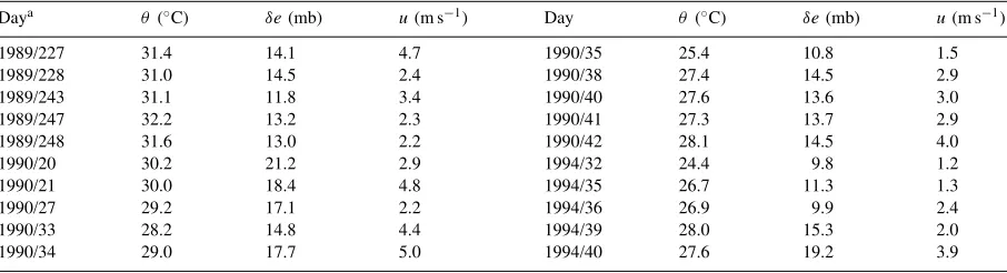
The data analysis involved the estimation of day-time (07:00–18:00 hours) values of (i) 20 min and hourly latent heat fluxes, (ii) average evaporation for the three periods of data collection and (iii) evapora-tion on individual days using Eq. (6), and followed by comparisons with the corresponding measured values. The 20 min and hourly values of latent heat flux were estimated using a data set formed by combining data from all the three periods, January to February of 1994, January to February of 1990 and August to September of 1989. The individual days used in the calculations are listed in Table 3 including daytime average air temperature (θ), vapor pressure deficit (δe) which is equal to (e*−e) and wind speed (u). The days listed in Table 3 had data for at least 8 h during daytime. Two values for the parameterα′in Eq. (6) were used in the
calculations andβ was kept at 20 W m−2. One value
ofα′
was 0.95, which was the average value deduced by De Bruin and Holtslag (1982) using daytime hourly values of latent heat flux for their normal period, and the other was 1.05. The motivation for testing 1.05 for α′ was the following. As stated in the study of
De Bruin and Holtslag (1982), Priestley–Taylor pa-rameter α and the parameterα′ have shown similar
behavior and daily mean value ofαhas appeared to be about 10% greater than its hourly value during day-time. Therefore we could expectα′to be about 10%
greater when daily values are considered, for a given
β. Thus, it is justified to test the value of 1.05 forα′.
For further evaluation of the results, we estimated (i) daytime evaporation on days listed in Table 3 using
Table 3
Mean values of daytime temperature (θ), vapor pressure deficit (δe) and wind speed (u) for selected days
Daya θ (◦C) δe(mb) u(m s−1) Day θ (◦C) δe(mb) u(m s−1)
1989/227 31.4 14.1 4.7 1990/35 25.4 10.8 1.5
1989/228 31.0 14.5 2.4 1990/38 27.4 14.5 2.9
1989/243 31.1 11.8 3.4 1990/40 27.6 13.6 3.0
1989/247 32.2 13.2 2.3 1990/41 27.3 13.7 2.9
1989/248 31.6 13.0 2.2 1990/42 28.1 14.5 4.0
1990/20 30.2 21.2 2.9 1994/32 24.4 9.8 1.2
1990/21 30.0 18.4 4.8 1994/35 26.7 11.3 1.3
1990/27 29.2 17.1 2.2 1994/36 26.9 9.9 2.4
1990/33 28.2 14.8 4.4 1994/39 28.0 15.3 2.0
1990/34 29.0 17.7 5.0 1994/40 27.6 19.2 3.9
aDay is given as: year-day number.
Penman (1948) scheme given by (1) withf(u) from Eq. (2) and Priestley and Taylor (1972) scheme given by Eq. (4) with 1.26 and (ii) daytime 20 min and hourly values of latent heat flux using Eq. (5) withα=1.26 for the combined data set. The values estimated were compared with the corresponding measured values.
A value of 0.674 mb K−1 was used for γ in the
analysis. This value corresponds top=1014 mb (av-erage measured pressure), cp=1005 J kg−1K−1 and λ=2.43×10⁶J kg−1 (Brutsaert, 1982). The values of 1ande* were estimated employing Lowe’s polyno-mials (Lowe, 1977) for1ande*, and our air temper-ature measurements.
6. Results and discussion
Table 4 presents the linear regression results from the comparison of the measured 20 min and hourly la-tent heat flux with the corresponding values estimated using Eq. (6) and Priestley and Taylor (1972) scheme withα=1.26. The first value inside the parentheses
in every column corresponds toα′
=1.05 and the
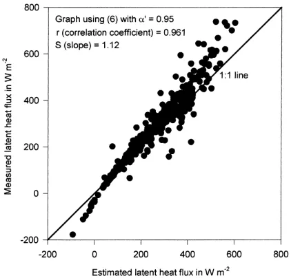
sec-ond value is from Priestley and Taylor (1972) scheme withα=1.26. The value outside the parentheses cor-responds toα′=0.95. Figs. 1 and 2 illustrate the
com-parison of hourly values for α′ =0.95 and α′=1.05,
respectively. The results in Table 4 show that for the 20 min and hourly time steps, the correlation coeffi-cients are better than 0.95 for all the cases considered, indicating good correlation between the measured values and the values estimated using Eq. (6) with
Table 4
Linear regression results of the comparison between the measured latent heat flux and the estimated flux using (i) De Bruin and Holtslag scheme given by Eq. (6) and (ii) Priestley–Taylor scheme given by Eq. (5) withα=1.26
Quantitya 20 min values Hourly valuesb
M 1639 423
Yav(W m−2) 256.2 284.2
S 1.11 (1.0, 0.83) 1.12 (1.02, 0.84) I(W m−2) −5.7 (−3.6, 16.4) −8.4 (−6.2, 14.6) η(W m−2) 56.5 (51, 68) 50.8 (42, 60.4)
r 0.954 0.961
η/Yav (%) 22 (20, 26) 18 (15, 21) aM=number of data values, S=slope, I=intercept,
Yav=average measured latent heat flux, r=correlation coeffi-cient and η=root mean square error given by: {6(measured value−estimated value)2/M}1/2. The first value inside parentheses
is from Eq. (6) withα′
=1.05 and the second value is from Eq. (5) withα=1.26. The value outside the parentheses is from Eq. (6) withα′
=0.95. The data set used is the combination from the three periods of data collection.
bHourly values refer to average of three successive 20 min
values within 1 h.
slopes and the root mean square errors, however, show differences. For both time steps, the application of Eq. (6) has produced slopes greater than 1.0. Based on the closeness to 1.0, values for the slope withα′
=1.05 are
Fig. 1. Comparison of the measured daytime hourly latent heat flux with the flux estimated using Eq. (6) andα′
=0.95, for the combined data set.
Fig. 2. Comparison of the measured daytime hourly latent heal flux with the flux estimated using Eq. (6) andα′=1.05, for the
combined data set.
better than those with 0.95. The improvement is about 11% and it is visible in Figs. 1 and 2, especially at high
lvalues. The root mean square errors as a percentage of the measured average values are smaller than 22% with 2–3% improvement by the use of 1.05 forα′
. It is seen from the results in Table 4 that the use of Eq. (5) withα=1.26 has produced slopes (0.84 and 0.83) which are much smaller (about 17%) than 1.0 and root mean square errors higher (3–6%) than those resulted by the use of Eq. (6). The slope values much smaller than 1.0 is an indication of the fact that the val-ues estimated by Eq. (5) withα=1.26 are higher than the measured values, on the average. This implies that the blending of data from different periods and hours has resulted in a data set that corresponds to a situa-tion where the average surface moisture level is below saturation. This type of situation is useful in testing Eq. (6) because the period of study in De Bruin and Holtslag (1982) for whichα′=0.95 andβ=20 W m−2
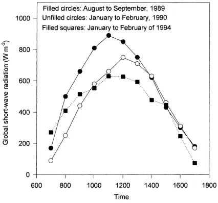
Fig. 3. Daytime variation of the global short-wave radiation for the periods: August to September of 1989, January to February of 1990 and January to February of 1994.
coefficient and the root mean square error obtained by applying Eq. (6) andα′=0.95 with the corresponding
De Bruin and Holtslag (1982) values indicates that our results are closer (within 1%) to theirs. The correla-tion coefficient obtained by them was 0.97 and the root mean square error was 17% of the average measured hourly latent heat flux. A comparison of our measured average latent heat flux with the average latent heat flux of De Bruin and Holtslag (1982), for hourly val-ues, shows that our value (284 W m−2) is 2.27 times
greater than theirs (125 W m−2). The latent heat flux
levels in the tropics are higher because of higher ra-diation levels, shown in Fig. 3. The above results in-dicate that the skill of De Bruin and Holtslag (1982) scheme is consistent even at higher flux levels and slightly wetter conditions (our average value forαis greater than theirs by 5%).
Table 5
Daytime (07:00–18:00 hours) measured average evaporation and estimated values using Eq. (6) with α′
=0.95 and 1.05, for the three periods of data collectiona
Quantity August–September 1989 January–February 1990 January–February 1994
E(mm), measured 4.21 3.65 2.89
E(mm), using Eq. (6) withα′=0.95 3.73 (11.4%) 3.35 (8.2%) 2.87 (<1%)
E(mm), using Eq. (6) withα′
=1.05 4.09 (2.8%) 3.68 (<1%) 3.14 (8.7%)
aThe percentages inside the parentheses are the deviations from the measured values.
Table 5 presents daytime average evaporation mea-sured and calculated using Eq. (6) withα′
=0.95 and
1.05 for the three data collection periods. The percent-age deviations (given inside the parentheses) are less than 11.4% with α′=0.95 and 8.7% with α′=1.05.
These results indicate that Eq. (6) satisfactorily esti-mates daytime average evaporation over larger time steps of the order of several days, 28–32 days, and
α′=1.05 provides better results. The improvement in
August to September of 1989 and January to Febru-ary of 1990 by the use ofα′=1.05 in Eq. (6) is more
than the offset in January to February of 1994. The percentage deviation (d) as used in our work is given by Eq. (14).
d=100×measured value−estimated value
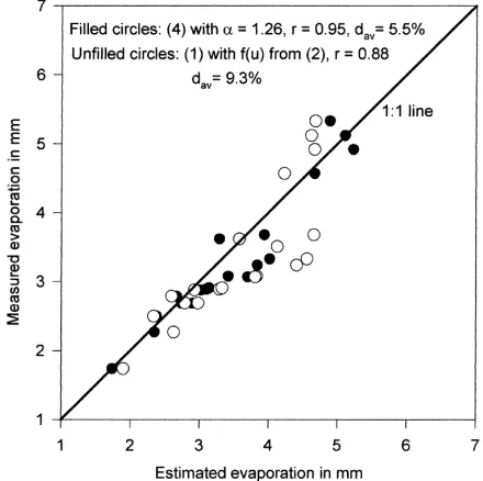
measured value (14) Table 6 presents the results from the comparison of estimated daytime evaporation with the correspond-ing measured values on individual days listed in Table 3. The evaporation was estimated using (i) De Bruin and Holtslag (1982) scheme withα′=0.95 and 1.05,
(ii) Priestley and Taylor (1972) scheme withα=1.26 and (iii) Penman (1948) scheme given by Eq. (1) with
Table 6
Results from the comparison of daytime measured evaporation and evaporation estimated using (i) De Bruin and Holtslag scheme given by Eq. (6) withα′=0.95 and 1.05, (ii) Priestley–Taylor scheme, given by Eq. (4) withα=1.26 and (iii) Penman scheme, given by Eq. (1)
withf(u) from Eq. (2), for the days in Table 3 Quantitya Eq. (6) withα′
=0.95 Eq. (6) withα′
=1.05 Eq. (4) withα=1.26 Eqs. (1) and (2)
S 1.27 1.15 0.95 0.91
I(mm) −0.34 −0.32 0.02 0.08
r 0.95 0.95 0.95 0.88
η(mm) 0.566 0.365 0.347 0.584
Eav (mm) 3.34 3.34 3.34 3.34
η/Eav (%) 17 11 10 17
dav (%) 12.2 3.8 5.5 9.3
aThe definitions of the quantitiesS,I,r, andη are the same as those in Table 4, except that the analysis is for the evaporationE.
Eav=average of measured evaporations anddav=average of percentage deviations.
are satisfactory but there is good (6–8%) improve-ment in the root mean square error value and average percentage deviation withα′=1.05. The improvement
is visible in Fig. 4. Regarding the improvement and the use of 1.05 forα′, it is necessary to mention that
in a few cases (4 out of the 20) the use of 1.05 for
α′
worsened the percentage deviation by about 4%. But this offset was tolerable compared to the overall improvements produced. (iii) The level of agreement between values estimated by Eq. (1) with f(u) from
Fig. 4. Comparison of the daytime measured evaporation on days given in Table 3 with values estimated using Eq. (6).
Eq. (2) and measured values is acceptable, but lower than the level of agreement from the use of Eqs. (4) or (6). This indicates that Eq. (6) with α′=1.05 or
Eq. (4) withα=1.26 are better choices for estimat-ing daytime evaporation on a daily basis for the type of study we conducted. However, from Fig. 5 it can be seen that on some days (about 6) percentage devi-ations are small, less than about 6%, indicating that the conditions had been favorable for potential evapo-transpiration.
The results from Eq. (4) with α=1.26 and those
from Eq. (6) with α′
=1.05 are very close as seen
in Table 6. Therefore, it appears that Eq. (4) with
α=1.26 is as equally good as Eq. (6) with α′=1.05
for estimating daytime evaporation on a daily basis in practice. But a careful analysis will indicate that Eq. (6) withα′=1.05 or 0.95 may be better in practical
ap-plications. A closer look at Figs. 4 and 5 reveals that, the days on which Eq. (4) withα=1.26 produces large negative percentage deviations are well modeled by Eq. (6) withα′=1.05 or 0.95. Higher negative
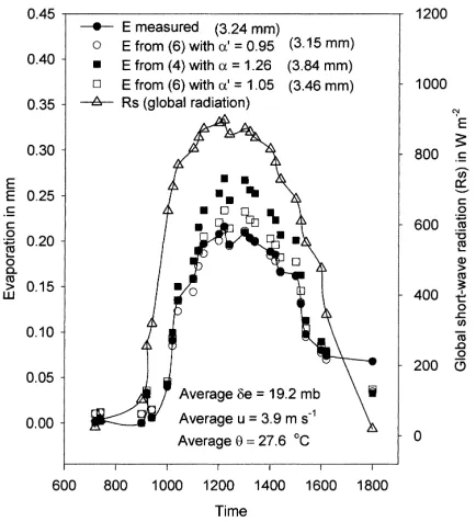
percent-age deviations imply larger overestimates for evapo-ration by Eq. (4) and indicate below satuevapo-ration surface moisture conditions. These conditions normally exist in practice, especially on agricultural lands. Such sit-uations can be better described, including the daytime variation of evaporation, by Eq. (6) as the example in Fig. 6 illustrates. Fig. 6 shows the daytime variation of evaporation in 20 min time steps for the 40th day of January 1994. Evaporation measured, evaporation calculated using Eq. (4) with α=1.26, evaporation calculated using Eq. (6) with α′=0.95 and
Fig. 6. Daytime variation of global short-wave radiation, evapora-tion measured, evaporaevapora-tion estimated using Eq. (6) withα′
=0.95 and 1.05, and Eq. (4) withα=1.26, for the 40th day of January 1994. The total evaporation values are given inside parentheses.
tion calculated using Eq. (6) withα′
=1.05 are shown
as a function of time. The graphs show that Eq. (6) models the variation well, but Eq. (4) fails (d=18.6%) especially around mid-day. The daytime evaporation estimated using Eq. (6) agree well with the measured value. The percentage deviation with α′=0.95 was
2.8% and the percentage deviation withα′=1.05 was
6.8%, which are good. Apparently, this day was one of the days for which the value 1.05 forα′produced an
offset of 4%. This type of departure of the evaporation estimated using Eq. (4) withα=1.26, around mid-day, was also observed with other days having higher percentage deviations. A reason can be the surface moisture depletion due to higher evaporation around mid-day influenced mainly by radiation. For the 40th day of January 1994, the variation of the global short-wave radiation is also shown in Fig. 6. The global short-wave radiation around noon on this day is about 850 W m−2. Evaporation around mid-day is
about 0.225 mm for 20 min. There is good correlation between evaporation and radiation. The correlation coefficient between evaporation and global short-wave radiation for this day is 0.91. Apart from radiation, the other factors that can influence evaporation are vapor pressure deficit and wind speed. The average values of daytime vapor pressure deficit and wind speed for the 40th day of January 1994 were 19.2 mb and 3.9 m s−1,
respectively. The correlation coefficients for the com-parison of evaporation with vapor pressure deficit and wind speed on this day were 0.89 and 0.73, respec-tively, which indicate that radiation has a stronger influence on evaporation followed by vapor pressure deficit. Further studies, however, are necessary to substantiate our observations on moisture depletion.
7. Concluding remarks
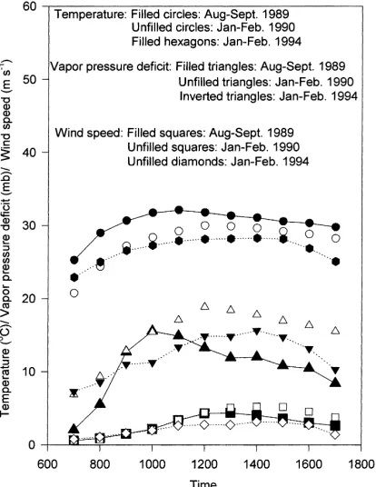
Fig. 7. Daytime variation of hourly average values of temperature (θ), vapor pressure deficit (δe) and wind speed (u), during the three periods of data collection.
deficit and wind speed given in Figs. 3 and 7 are day-time hourly average values. The phrase dayday-time hourly average values refer to the averages for each hour be-tween 07:00 and 18:00 hours, during any period un-der review. From Figs. 3 and 7 it is seen that radiation levels, temperatures and vapor pressure deficits have been different during the three periods with August to September of 1989 having higher radiation levels and temperatures than January to February periods. Mid-day radiation levels in August to September is higher by about 250 W m−2, on the average, and the
temperature is higher by about 3◦C. Generally, May to
November period is warmer and December to Febru-ary is colder in Jamaica. On the other hand, vapor pres-sure deficit in August to September is lower by about 4 mb, on the average, than January to February values with January to February of 1990 having a higher va-por pressure deficit, about 18 mb around mid-day. The wind speeds were close to one another. The difference in the wind speeds was smaller than 1 m s−1. The
re-sults from our study indicated that De Bruin and
Holt-slag (1982) scheme predicts latent heat flux and evapo-ration well under the conditions existed in Jamaica and behaves well over different time steps. The scheme is suitable for estimating latent heat flux and evaporation from regularly watered fields with short grass (short crops) in tropical regions with environmental condi-tions similar to those existed in Jamaica. The value 1.05 for the parameterα′ may improve the results.
Acknowledgements
The authors are thankful to Mr. N. Thomas of the Physics Department, UWI, Mona campus for the help rendered towards setting up of the experiment sta-tion, data collection and participation in the discus-sions meant to resolve instrumentation problems. The constructive suggestions and thoughtful comments of the reviewers are gratefully appreciated.
Appendix A. Calculation ofLLL
Monin–Obukhov lengthLwas determined by itera-tion using Eqs. (A.1)–(A.5) given later. Within about five iterations it was possible to obtainLvalues with a deviation less than 1%. Eqs. (A.1)–(A.5) are from Brutsaert (1982), Dyer (1974), Businger (1988), Par-lange and Katul (1992). The values of L calculated were hourly average values using measured hourly av-erage values of l, H, u, e and Ta. Eqs. (A.3)–(A.5)
presented here assume that the zero plane displace-ment height, do, is small compared to the
measure-ment height of 2 m
L= −u∗
3
[kgHv/ρcpTa]
(A.1)
whereg=9.8 m s−2, c
p is the specific heat of air at
constant pressure,Ta the air temperature inK,ρ the
density of air,kvon Kármán’s constant (0.4),u* the friction velocity and Hv=(H+0.61cpTa l/λ) is the specific flux of virtual sensible heat. The units of the quantities are such thatL in Eq. (A.1) is in m. The densityρ is given by
ρ=
p
RdTa 1−
0.378e p
wherep is the atmospheric pressure,Rdthe gas
con-wherezois the momentum roughness length and was
taken to be equal to 0.023 m (Brutsaert, 1982) and
ψm is the momentum stability correction function
which is given by Eq. (A.4) below for unstable atmo-spheric conditions. For stable atmoatmo-spheric conditions
ψmgiven in Eq. (A.5) was used.
The procedure for calculation of Lvalue for a given set of values ofl,H,e,uandTawas as follows. With
an initial guess for L, u* was estimated from Eq. (A.3). With thisu*, a first value forLwas calculated from Eq. (A.1) and this L value was compared with the initial guess forL. The firstLvalue calculated was then used in Eq. (A.3) to determine a newu* which led to a second Lvalue from Eq. (A.1). The process continued until theLvalue calculated using Eq. (A.1) was within about 1% of the previousLvalue.
References
Brutsaert, W., 1982. Evaporation into the atmosphere. Reidel, Dordrecht, 299 pp.
Brutsaert, W., Stricker, H., 1979. An advection-aridity approach to estimate actual regional evapotranspiration. Water Resources Res. 15 (2), 443–450.
Businger, J., 1988. A note on the Businger–Dyer profiles. Boundary Layer Meteorol. 42, 145–151.
Campbell Scientific Inc., 1987. CSI eddy correlation and Bowen ratio instrumentation preliminary instruction manual, 28 pp. Cargo, R.D., Brutsaert, W., 1992. A comparison of several
evaporation equations. Water Resources Res. 28 (3), 951– 954.
Chen, A.A., 1992. Evaporation modelling in Jamaica. Jam. J. Sci. Technol. 3, 41–46.
Chen, A.A., Daniel, A.R., Daniel, S.T., Gray, C.R., 1990. Wind power in Jamaica. Solar Energy 44 (6), 355–365.
De Bruin, H.A.R., Holtslag, A.A.M., 1982. A simple parameterization of the surface fluxes of sensible and latent heat during daytime compared with the Penman–Monteith concept. J. Appl. Meteorol. 21, 1610–1621.
Dyer, A.J., 1974. A review of flux-profile relationships. Boundary Layer Meteorol. 7, 363–372.
Eichinger, W.E., Parlange, M.B., Stricker, H., 1996. On the concept of equilibrium evaporation and the value of the Priestley–Taylor coefficient. Water Resources Res. 32 (1), 161–164.
Hsu, S.A., 1982. Determination of the power-law wind profile exponent on a tropical coast. J. Appl. Meteorol. 21, 1187– 1190.
Katul, G.G., Parlange, M.B., 1992. A Penman–Brutsaert model for wet surface evaporation. Water Resources Res. 28 (1), 121– 126.
Konzelmann, T., Calanca, P., Mü1ler, G., Menzel, L., Lang, H., 1997. Energy balance and evapotranspiration in a high mountain area during summer. J. Appl. Meteorol. 36, 966–973. Lowe, P.R., 1977. An approximating polynomial for the
computation of saturation vapor pressure. J. Appl. Meteorol. 16, 100–103.
Monteith, J.L., 1965. Evaporation and environment. The state and movement of water in living organisms, Symp. Soc. Exp. Biol. 19, Academic Press, NY, pp. 205–234.
Ohmura, A., 1982. Objective criteria for rejecting data for Bowen ratio flux calculations. J. Appl. Meteorol. 21, 595–598. Parlange, M.B., Katul, G.G., 1992. An advection-aridity
evaporation model. Water Resources Res. 28 (1), 127–132. Penman, H.L., 1948. Natural evaporation from open water, bare
soil and grass. Proc. R. Soc. London A193, 120–145. Priestley, C.H.B., Taylor, R.J., 1972. On the assessment of surface
heat flux and evaporation using large-scale parameters. Monthly Weather Rev. 100, 81–92.