Transport of waste leakage in stratified
formations
Hongbin Zhan
Department of Geology and Geophysics/MS 3115, Texas A&M University, College Station, TX 77843-3115, USA
(Received 17 April 1997; revised 10 November 1997; accepted 22 December 1997)
Contaminant transport in a strongly heterogeneous stratified formation whose log hydraulic conductivity distribution has a variance greater than unity is investigated. Four kinds of waste leakage scenario are studied. They are: (1) continuous waste leakage from landfills; (2) temporal waste leakage from landfills; (3) continuous deep-well injection wastes; and (4) temporal deep-deep-well injection wastes. Ensemble average concentrations and variances of concentration distributions are calculated for the four scenarios. The results in this paper show that when heterogeneity of a formation increases, transport in this formation differs significantly from the linear solutions which assume that the variances of log hydraulic conductivity are less than unity. q1998 Elsevier Science Limited. All rights reserved
Keywords: strongly heterogeneous, waste disposal, contaminant transport, stratified formations.
1 INTRODUCTION
Underground waste disposal is used for industrial and domestic wastes in many places around the world. Owing to complex subsurface geology and associated heterogene-ities, the leakage of waste from a storage site is often carried off site by groundwater. In addition, strong macrodispersion in the subsurface can expand an originally small plume to a very large volume. Efficient management of waste disposal requires a better understanding of contaminant transport in the subsurface, a subject which has been investigated exten-sively over the last 20 years. A reliable risk assessment of hazardous waste disposal also depends on a reliable estimation of contaminant concentration distribution in groundwater. One of the tools available to study con-taminant transport in the subsurface is the stochastic approach, which assumes that some of the hydrologic para-meters are spatially random variables. In order to achieve mathematically tractable solutions, a small perturbational approximation is usually employed. That is, the hydraulic conductivity changes mildly in space. Such an approach is often called the linear solution. For instance, linear solutions of nonreactive tracer transport have been performed by Gelhar et al.,9 Gelhar and Axness10 and Dagan;6 linear
solutions of the reactive tracer transport have been reported by Rubin,16Valocchi21and Bahr.2The linear solutions suc-cessfully describe the flow and transport processes in mildly fluctuating heterogeneous formations. Its extension to a strongly heterogeneous medium is still a research topic. Computer simulations have demonstrated that discrepancies exist between Monte Carlo simulation results and the results of linear theory.4,19,20,3,17In this paper, strong heterogeneity refers to a formation whose natural log hydraulic conduc-tivity distribution has a variance greater than unity. It is known that many field acquifers and geological formations have a wide range of hydraulic conductivity distributions which intrinsically require a nonlinear approach. The non-linear approach should include higher-order approximations of parameters to take into account the strong heterogene-ities. In recent years, several researchers have investigated groundwater flow and contaminant transport in strongly heterogeneous formations. Neuman and Zhang14 and Zhang and Neuman22 developed a quasi-linear theory to account for nonlinearity caused by a deviation of plume ‘particles’ from their mean trajectory calculated on the basis of a Lagrangian linear approach. Dagan8 introduced a second-order correction to transverse macrodispersivity based on his previous Lagrangian framework.6,7 Hsu et
Printed in Great Britain. All rights reserved 0309-1708/98/$ - see front matter
PII: S 0 3 0 9 - 1 7 0 8 ( 9 8 ) 0 0 0 0 1 - 3
al.12presented a higher-order study on flow and transport in strongly heterogeneous formations based on the quasi-linear theory of Neuman and Zhang.14
Several other researchers have explored alternative theories to investigate the fluid flow and contaminant trans-port in strongly heterogeneous formations. For example, Christakos and others5have used diagrammatic analysis to resolve the complex multifold integrals that appear in the perturbative expansion of the stochastic flow solution and the numerical performance of the approach is tested. Serrano18has reformulated the flow and transport equations through the aid of the Adomains Decomposition Method.1A great deal of research opportunities exist in these alternative nonlinear theories.
In this paper, an attempt is made to solve the problems of transport in strongly heterogeneous formations without using a small perturbational framework. The stochastic transport equations are solved to obtain solutions for (1) the ensemble average concentrations and (2) the variances of concentration. In this analysis, local-scale dispersivity and diffusion are neglected based on the consideration that the primary cause of field dispersion is field hetero-geneity. Also, the mathematical manipulation is simpler when local dispersivity and diffusion are neglected. We are aware that neglecting the local dispersivity will cause a loss of information on the transverse mixing of the solute and absence of the spatial correlation of hydraulic conduc-tivity. Including the local dispersivity effect in the nonlinear framework is a future research topic and is not discussed in this paper. The investigation in this paper focuses on the transport of leakage from two kinds of waste disposal schemes: (1) landfills in a formation with a uniform ground-water flow direction; and (2) deep-well injection. Four kinds of leakage transport problem will be investigated: (1) continuous leakage; (2) temporal leakage; (3) continuous injection; and (4) temporal injection. The work presented in this paper can help us gain more insight into the sophisticated transport process in strongly heterogeneous formations. It is the first step towards buiding a nonlinear framework of contaminant transport in a three-dimensional, heterogeneous formation.
2 TRANSPORT OF WASTE LEAKAGE FROM A LANDFILL SITE
2.1 Continuous waste leakage from a landfill site
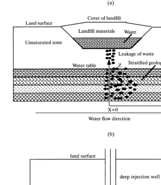
A simplified physical view of leakage from a landfill into a stratified formation is shown in Fig. 1(a). The dispersion of waste leakage in the unsaturated zone is not included. Con-taminant leakage with constant concentration is released at
x¼0 in all layers. The stratigraphy is horizontal such that the hydraulic conductivity does not change along thexaxis but does change along the vertical direction (zaxis). Uni-form groundwater flow is from left to right, parallel with the stratigraphic layers. Constant head boundary conditions are
applied on the left and right sides, so that the head gradient is constant throughout the model. We should point out that the constant head boundary is only one possible condition of the regional groundwater flow. We impose these boundary conditions to isolate the effect of heterogeneity and to con-duct sensitivity tests of the contaminant transport upon the heterogeneity. Because of different hydraulic conductivities in different layers, groundwater flow velocities are different in different layers. Stationarity of log conductivity is assumed throughout this work for both the landfill and the deep-well injection configurations, therefore, the ensem-ble average concentration is not dependent on zsince the layers are statistically identical; rather, it depends onxand timet.
It is generally accepted that, for nonreactive solute trans-port in a region without sinks/sources, the concentration distribution is governed by the Advective-Dispersion Equa-tion (ADE) in a local scale:
=·(D·=C¹qC)¼]nC
]t (1)
where D is the local-scale dispersion coefficient tensor, which is determined by local-scale pore space geometry (grain size, shape, orientation, etc.) and groundwater flow velocity; q is groundwater discharge which is related to groundwater velocity V ¼ q/n, where n is porosity, C is concentration, t is time. Considering the limited informa-tion about hydraulic conductivity, a stochastic approach is used to treat the local-scale ADE as a stochastic partial differential equation. In a strongly heterogeneous acquifer containing different layers with different hydraulic conduc-tivities, the dispersive effect caused by velocity distribution will be the leading cause of dispersion. Local-scale disper-sion will cause some transverse mixing between different layers. On the basis of this consideration, the local disper-sive term in eqn (1) is neglected and the porosity n is assumed to be constant. This results in:
][V(z)C(x,z,t)]
]x ¼
]C
]t (2)
For a continuous leakage problem with a constant source concentration, the boundary condition is C(0,z,t) ¼ C0
and the initial condition is C(x,z,0) ¼ C0 for x # 0 and
Cðx;z;0Þ ¼0 forx$0. The solution of this stochastic equa-tion is a step funcequa-tion:
C(x,z,t)¼C0S[V(z)t¹x] (3) where the step functionS(x)¼1 forx$0 andS(x)¼0 for
x,0. From Darcy’s law, the velocity Vis:
V¼ ¹ K
n
dh
dx (4)
If constant head boundary conditions are applied at both sidesx¼0 andx¼L, we assign the variable
J¼ ¹ 1
n
dh
dx (5)
so thatJis constant for all layers. In this way, the randomness
of V is determined by the randomness of K. In general, ln(K) is assumed to be a normal distribution with a known mean and variance. The stochastic term ln(K) is split into a mean part F and a random part f, where
lnðKÞ ¼Fþf, and eqn (4) changes to
V¼KJ¼eFþfJ (6) The probability density function (pdf) of f is the well-known normal distribution with variancej2f:
p(f)¼ 1
2p p
jf
exp ¹ f
2
2j2f !
(7)
Now, the ensemble average of concentrationCis
¯ C¼
Z`
¹`C0S(Vt¹x)p(f)df (8)
Considering the property of the step function S, the inte-grand of eqn (8) is a nonzero term only whenVt¹x$0, which means that
Vt¹x¼eFþfJt¹x$0 (9)
Solving the inequality (9) we get
f $ln(x=Jt)¹F (10) The inequality (10) implies that the lower limitation of integration in (8) can be replaced by ln(x/Jt)¹F and eqn (8) becomes
¯ C¼
Z`
ln(x=Jt)¹FC0S(Vt¹x)p(f)df
¼C0
2 erfc
ln(x=Jt)¹F
2
p jf
" #
ð11Þ
where the complementary error function, erfc, is defined as
erfc(x)¼ 2
p p
Z`
xe
¹y2
dy (12)
The average velocity is
¯
V¼KJ¼eFþfJ¼eF
exp j2f=2
ÿ
J (13)
where
ef¼exp j2 f=2
ÿ
is obtained from a general property of the moment-gener-ating function15efq: E e fq
¼exp f¯qþj2fq2=2
, where E[] is the expectation sign, f is a Gaussian distribution with meanf¯ and variance j2f and qis a constant. The average travel distance is
¯
x¼Vt¯ ¼eFJexp j2f=2
ÿ
t (14)
eqn (11) becomes:
¯ C¼C0
2 erfc
lnðx=x¯Þ
2
p jf
þ jf
2p2
" #
(15)
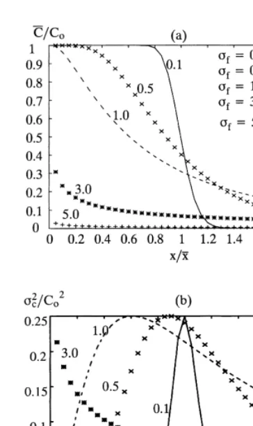
At a fixed time (x¯ is fixed),Cversusx=x¯ is plotted in Fig. 2(a) which is the breakthrough curve.
The variance of concentration isj2c¼C2¹ C¯
ÿ 2
. Similar to the calculation processes from eqns (8)–(11), we have
C2¼ Z
`
¹`C
2
0S2(Vt¹x)p(f)df
¼C
2 0 2 erfc
lnðx=x¯Þ
2
p jf
þ jf
2p2
" #
ð16Þ
j2c¼C2¹C¯ 2
¼C
2 0 2 erfc
lnðx=x¯Þ
2
p jf
þ jf
2p2
" #
¹C
2 0 4 erfc
2 lnðx=¯xÞ
2
p jf
þ jf
2p2
" #
ð17Þ
The normalized variances of concentration as functions of
x=x¯ (time is fixed) are plotted in Fig. 2(b).
Several interesting results are illustrated in Fig. 2(a) and Fig. 2(b):
1. Fig. 2(a) shows that when jfis very small (¼0.1), the point with C¯¼C0=2 is located approximately at
x¼x¯ (this point is usually called the 50% concentra-tion point or C50%). However, when heterogeneity increases jf increases, and the C50% point moves towards the source point (x ¼ 0) of contamination. TheC50%point is decided by the geometrical mean of hydraulic conductivity, K¯G¼eln(
K)
¼eF (see eqn (11)), while the average travel distance x¯ is decided by the arithmetical mean of hydraulic conductivity,
¯
K¼eF exp j2f=2
ÿ
¼K¯Gexp j2f=2
ÿ
(see eqn (14)). Thus K¯=K¯G¼exp j2f=2
ÿ .
1. Whenjfincreases, K¯G is smaller than K¯ and the difference between K¯ and
¯
KG gets larger, thus C50% point moves further from
x¼x¯ to the left in Fig. 2(a).
2. Fig. 2(b) shows that the point of maximal variance of concentration is close to x¼x¯ when the medium is nearly homogeneous (jf¼0.1). Therefore, usingC¯ as the concentration estimator has maximal uncertainty at the pointx<x¯whenjf¼0.1. The largest concen-tration variance is in the area where the mean concentration C¯ changes most rapidly; such a result has been pointed out by Gelhar11(p. 242). When jf increases, the maximal variance point shifts towards the origin in Fig. 2(b). This is because the point of maximal mean concentration gradient also moves towards the origin. Fig. 2(b) shows that the maximal variance isj2c=C20 ¼0.25 orjc/C0¼0.5.
3. Fig. 2(a) and Fig. 2(b) reveal that heterogeneity has a great impact on the concentration and variance of concentration distribution curves. Whenjfincreases, the corresponding concentration and variance of con-centration curves are deformed significantly from their counterparts forjf¼0.1.
2.2 Temporal waste leakage from a landfill site
In this section, contaminant transport with a temporal leak-age source is investigated. If the leakleak-age time isTand the other physical parameters are the same as those used in Section 2.1, the solution to the stochastic eqn (2) becomes
C¼ C0S[Vt
¹x]; if t,T
C0(S[Vt¹x]¹S[V(t¹T)¹x]); if t.T
(
(18)
Fig. 2.(a) Normalized concentration C=C¯ 0 as a function of x=x¯
(breakthrough curve); (b) normalized variance of concentration as a function ofx=x¯. ——,jf¼0.1; 3 3 3,jf¼0.5; – – –,jf¼
1.0; p p p,jf¼3.0.
The solution fort,Tis the same as that of Section 2.1, so onlyt . T is considered here. Following similar calcula-tions as those utilized in Section 2.1, the ensemble average concentration is
¯ C¼
Z`
¹`C0(S[Vt¹x]¹S[V(t¹T)¹x])p(f)df
¼C0
2 erfc
lnðx=x¯Þ
2
p jf
þ jf
2p2
" # (
¹erfc ln x= x¯¹x0
ÿ
2
p jf
þ jf
2p2
" #)
ð19Þ
wherex¯is the average travel distance given by eqn (14) and
x0 is defined as
x0¼VT¯ ¼eFJexp j2f=2
ÿ
T (20)
The variance of concentration is
j2c¼C2¹C¯ 2
¼C
2 0 2 erfc
lnðx=x¯Þ
2
p jf
þ jf
2p2
" # (
¹erfc ln x= x¯¹x0
ÿ
2
p jf
þ jf
2p2
" #)
¹C
2 0 4 erfc
lnðx=x¯Þ
2
p jf
þ jf
2p2
" # (
¹erfc ln x= x¯¹x0
ÿ
2
p jf
þ jf
2p2
" #)2
ð21Þ
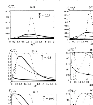
TheC¯=C0versusx=x¯andj2c=C20versusx=x¯curves are plotted in Fig. 3.
An interesting problem here is to see what happens when
the leakage time is very short (the so-called pulse source). In
By using the following approximation of the complemen-tary error function:
erfc(x)¹erfc(xþDx)< 2
eqns (19) and (21) are reduced to
¯
The macrodispersivity in a stratified aquifer was discussed by Gelhar11(pp. 204–207) and Dagan7(p. 293), so it is not repeated here. Our interest is to derive directly the concen-tration breakthrough curve, the variance of concenconcen-tration, and to test the sensitivity of these results with the variance of log conductivity. Gelhar11has derived the concentration for an instantaneous pulse source by recognizing that the travel time probability density function (pdf) is essentially equal to the normalized concentration. Although the physi-cal base of Gelhar’s analysis is correct, his eqn (5.1.14) is inaccurate and dimensionally inconsistent. As a matter a fact, in Gelhar’s analysis of (5.1.12), if we do one step further to transform the probability density functionfK to theflnK, we can easily derive the correct eqn (5.1.14) and find that it is identical to our solution (24). The mathema-tical process is shown below.
Recognizing that the notation ‘J’ used by us (see eqn (5)) equals ‘J/n’ used by Gelhar, his eqn (5.1.11) becomes
t¼ x
V¼ x
JK (26)
where t, V and K are the time, velocity, and hydraulic conductivity, respectively. By using Gelhar’s relationship (2.1.7), which is
fz(z)¼
If ln(K) obeys the normal distribution, from eqn (13) we have V¯ ¼elnK
eqn (28) is the accurate eqn (5.1.14) in Gelhar’s analysis. Remeber that
Z`
¹`cdt is the normalization factor which
equals the product of C0 and T used in Section 2.2,
¯
Vt¼x¯ and lnÿVt¯ =x¼ ¹lnðx=x¯Þ, then eqn (28) is identical to our solution (24). Therefore, Gelhar’s solution (eqn (5.1.14)) for a pulse source is a special case of our general solution (19) for any leakage timeT.
The following results are obtained in this section:
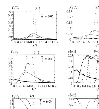
1. When T/t is small, for instanceT/t¼0.05 as in Fig. 3(a1), the leakage can be considered as a pulse source. Therefore, the concentration distribution has a bell shape. When T/t gets larger, the leakage time becomes longer, the scenario changes from a pulse source towards the continuous source, and the con-centration C¯=C0 distribution changes from a bell shape to the shape of continuous leakage (Section 2.1). Fig. 3(a1)Fig. 3(b1)Fig. 3(c1) exhibit the transi-tion from a pulse-type source to a continuous-type source. In Fig. 3(a1), the maximum C¯=C0 is about 0.2 when jf ¼ 0.1. It drops rapidly when jf gets larger because the concentration spreads over a wider range. The maximal C¯=C0 increases whenT/t gets larger for each of the cases ofjf¼0.1, 0.5, 1.0 and 3.0, because a longer leakage time will bring more solute into the aquifer and enhance the concentration. 2. Fig. 3(a2)Fig. 3(b2)Fig. 3(c2) are the variances of concentration for different leakage times. At an inter-mediate leakage time (Fig. 3(b2)), the variances of concentration show bidmodal (two peaks) shapes for
jf¼0.1, 0.5 and 1.0. Forjf¼3.0, the bimodal shape is not clearly shown in the Fig. 3(b2). Fig. 3(b1) shows that the concentration changes most rapidly in the two corners of the flat top for jf ¼ 0.1, thus there are two maximal peaks of concentration variances corresponding to these two corners. The rationale is still the same as addressed in point (2) of Section 2.1: the largest concentration variances occur in the areas where concentrations change most rapidly. The region between these two corners is a flat top where the concentration change is extre-mely small, so the concentration variance in that area is near zero as shown in the Fig. 3(b2) forjf¼0.1. WhenTis larger, the flat top region is wider, thus the distance between the two peaks of concentration variances is larger. For a strong heterogeneity, the concentration distribution spreads over a much
larger range; thus it is harder to see the flat top of the concentration distribution. That is why the bimodal distribution often seen for small jf is not shown for largejf. The bimodal shape of the variance of concen-tration has been studied before within a linear theory framework, for instance, by Kapoor and Gelhar15.
3 TRANSPORT OF WASTE DISPOSAL THROUGH DEEP INJECTION WELL
3.1 Continuous injection of waste
A simplified schematic diagram of waste disposal through a deep injection well is shown in Fig. 1(b). Since the flow field generated by the high injecting pressure is much stronger than regional growndwater flow, the regional groundwater flow will be neglected with the focus on the radial flow pattern caused by injection. The aquifer setting is exactly the same as used in Section 2: a stratified aquifer, where hydraulic conductivity varies in the vertical direction but does not change in the horizontal direction. Groundwater flow and solute transport are in symmetric radial patterns.
The steady-state groundwater flow is governed by equation
=2h¼0 (29)
The flow is radial so that headhis a function ofr(distance from the injection well). In this case, eqn (29) becomes
=2h¼1
With constant boundary conditions, the solution of eqn (30) is
h¼ ¹aln r=rw
ÿ
þb (31)
whereaandbare constants determined by pressures atr¼
rw and r¼ R respectively, where rw is the radius of the injection well andRis the influence radius of the injection well. Explicitly, aandbare:
a¼ h0¹hR
ln R=rw
ÿ , b¼h0 (32)
where h0 and hR are heads ar r ¼ rw and r ¼ R,
re-spectively. Eqn (32) shows that if waste is injected at high pressure (h0qhR), ‘a’ could be very large.
The radial flow velocity is then:
V(z)¼ ¹K=h=n¼a=n
r K(z)¼ a0
rK(z) (33)
where a0 ¼ a/n. The longitudinal macrodispersion in a
strongly heterogeneous aquifer is dominated by field het-erogeneity which causes velocity contrasts in the different layers. Local-scale dispersion is neglected. In a cylindrical coordinate system, the stochastic solute transport equation is:
=·(CV)þ]C
If the concentration at the injection well is a constantC0, the solution to eqn (34) also is a step function:
C¼C0S t¹
eqn (35) is different from the solution in Section 2 (eqn (3)). That is because the velocity in the radial flow is no longer a constant as was the case for uniform flow. Here, velocity is inversely proportional to r(see eqn (33)). The ensemble average of concentration is obtained through an equation of the same form as (8). Similar to the develop-ments in Section 2, the limit of integration is changed because the step function is nonzero only when
t¹ r
Changing the limit and performing the integration results in:
The average flow velocity is:
¯
The average travel distance can be obtained by solving dr
Thus the solution is
¯
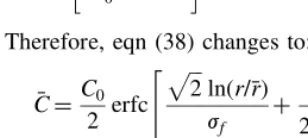
Therefore, eqn (38) changes to:
¯
The variance of concentration is calculated by using similar steps to those adopted in Section 2.
j2c¼ shown in Fig. 4(a). The normalized variances are exhibited in Fig. 4(b).
3.2 Temporal injection of waste
In Section 3.1, the waste was injected continuously into the ground. In this section, the waste is injected over a temporal time periodT. In this case, the solution to the stochastic eqn (34) is Section 3.1, so only t . T is considered. Similar to the manipulations of Section 3.1, the average concentration is
¯
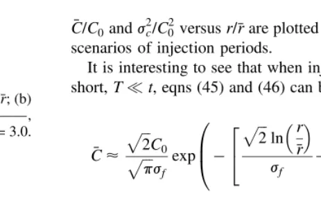
. The variance of concentration is scenarios of injection periods.
It is interesting to see that when injection timeTis very short,Tpt, eqns (45) and (46) can be reduced to
The following points appear to be noteworthy.
1. The normalized concentrationsC¯=C0and variances of concentrationj2c=C02 are similar to those in Section 2. 2. Eqn (47) shows that when T/t is small,C¯=C0 is pro-portional to (T/t)1/2. This result is different from its counterpart (T/t) in Section 2 (eqn (24)). That is because, in Section 3, flow is radial and the volume occupied by the leakage expands radially. At a given time and location, when leakage timeTincreases, the increasing rate of concentration should be lower than that in the unidirectional flow of Section 2.
Fig. 4.(a) Normalized concentrationC=C¯ 0as a function ofr=¯r; (b) normalized variance of concentration as a function ofr=¯r. ———,
jf¼0:1; 3 3 3,jf¼0.5; – – –,jf¼1.0; p p p,jf¼3.0.
4 DISCUSSIONS AND CONCLUSIONS
In this paper, we have derived the ensemble average con-centration breakthrough curves and the associated variances of the concentration of four different scenarios in stratified formations. The purpose is to show a nonlinear method-ology of solving the transport stochastic partial differential equation when the small perturbation assumptions of log conductivity are not valid. Sensitivity analyses are con-ducted that isolate the effect of aquifer heterogeneity and allow the investigation of cases of high variances. However, we should be aware that this is a first step towards the description of groundwater flow and contaminant transport in a strongly heterogeneous aquifer with large variances of log conductivity, which is currently a topic of great concern in the hydrologic science community. As recognized by Gelhar11 and many other researchers, the convective model in a stratified formation will lead to an exaggerated macrodispersity. A great deal of research is needed to obtain a three-dimensional description of transport in strongly heterogeneous formations in the future.
The following conclusions are drawn from this research.
1. The transport processes of waste disposal have been investigated in this paper. Closed-form analytical solutions of ensemble average concentrations and var-iances of concentration are obtained for four waste disposal scenarios: (i) continuous leakage from a landfill; (ii) temporal leakage from a landfill; (iii) continuous injection into an injection well; and (iv) temporal injection into an injection well. In this paper, stratified geological formations are assumed and local dispersion is neglected.
2. The results show that heterogeneity has a significant impact on the concentrations and variances of concen-tration distributions. The shapes of concenconcen-tration distributions and variances of concentration distribu-tions change significantly when jf increases. It appears that the point of C50% moves towards the
origin in the breakthrough curve when jf increases. The variance of concentration is large in the area
where concentration change is rapid. The
breakthrough curve has a bell shape and reaches a maximum around x<¯xin Section 2 orr<r¯in Sec-tion 3 whenjfis small. The bell shape becomes flat when heterogeneity increases because of the broad velocity distribution for strong heterogeneity. The maximal variance of concentration shifts towards the origin when jf increases. This is because the area of rapid concentration change also shifts towards the origin when jf increases. The upper limit of variance isjc/C0¼0.5.
3. In the temporal waste leakage or temporal waste injection scenario, the variances of concentration exhibit bimodal distributions at a certain range of leakage or injection time T. This is because the con-centrations change rapidly in two discrete locations at which variances of concentration reach their maxi-mum. The distance between the two peaks will increase as T gets larger. The bimodal characteristic of variance of concentration is not shown for strong heterogeneity because the concentration distribution is broad and a flat top region cannot be established. For a pulse source (T p t), the ensemble average concentration is proportional toT/tin the landfill sce-nario and proportional to (T/t)1/2 in the deep-well injection scenario.
ACKNOWLEDGEMENTS
I thank Drs Patrick Domenico and Mark Everett for their prereview of this manuscript before submission. I also thank the three anonymous journal reviewers for their comments on this manuscript. This research was supported by the Faculty Research Developing Fund, Faculty Mini-grant, and Research Enhancement Funds of the Texas A&M University.
REFERENCES
1. Adomian, G., Nonlinear Stochastic Operator Equations. Academic Press, New York, 1986.
2. Bahr, J. M., Analysis of nonequilibrium desorption of vola-tile organics during field test of aquifer decomposition. J. Contam. Hydrol., 1989,4,205–222.
3. Bellin, A., Salandin, P. and Rinaldo, A. Simulation of dis-persion in heterogeneous porous formations: statistics, first-order theories, convergence of computations.Water Resour. Res., 1992,28,2211–2227.
4. Chin, D. and Wang, T., An investigation of the validity of
first-order stochastic dispersion theories in isotropic porous media.Water Resour. Res., 1992,28,1531–1542.
5. Christakos, G., Hristopulos, D. T. and Miller, C. T., Stochastic diagrammatic analysis of groundwater flow in heterogeneous porous media.Water Resour. Res., 1995,31,
1687–1703.
6. Dagan, G., Solute transport in heterogeneous porous forma-tions.J. Fluid Mech., 1984,145,151–177.
7. Dagan, G., Flow and Transport in Porous Formations. Springer-Verlag, Berlin, 1989.
8. Dagan, G., An exact nonlinear correction to transverse macrodispersivity for transport in heterogeneous formations. Water Resour. Res., 1994,30,2699–2705.
9. Gelhar, L. W., Gutjahr, A. L. and Naff, R. L., Stochastic analysis of macrodispersion in a stratified aquifer. Water Resour. Res., 1979,15,1387–1397.
10. Gelhar, L. W. and Axness, A. C., Three-dimensional stochas-tic analysis of macrodispersion in aquifers. Water Resour. Res., 1983,19,161–180.
11. Gelhar, L. W., Stochastic Subsurface Hydrology. Prentice Hall, Englewood Cliffs, NJ, 1993.
12. Hsu, K.-C., Zhang, D. and Neuman, S. P., High-order effects on flow and transport in randomly heterogeneous porous media.Water Resour. Res., 1996,32,571–582.
13. Kapoor, V. and Gelhar, L. W., Transport in three-dimension-ally heterogeneous aquifers, 2. Predictions and observations of concentration fluctuations.Water Resour. Res., 1994,30,
1789–1801.
14. Neuman, S. P. and Zhang, Y.-K., A quasi-linear theory of non-Fickian and Fickian subsurface dispersion, 1, Theoreti-cal analysis with application to isotropic media. Water Resour. Res., 1990,26,887–902.
15. Ross, S. M., Introduction to Probability Models, 5th edn. Academic Press, San Diego, CA, 1993.
16. Rubin, J., Transport of reacting solutes in porous media: relation between mathematical nature of problem formula-tion and chemical nature of reacformula-tions. Water Resour. Res., 1983,19,1231–1252.
17. Salandin, P. and Rinaldo, A., Numerical experiments on dis-persion in heterogeneous porous media. In Computational Methods in Subsurface Hydrology, ed. G. Gambolati et al. Springer-Verlag, New York, 1990.
18. Serrano, S. E., Towards a nonperturbation transport theory in heterogeneous aquifers.Math. Geol., 1996,28,701–721. 19. Tompson, A. F. B. and Gelhar, L. W., Numerical simulation
of solute transport in three-dimensional, randomly hetero-geneous porous media. Water Resour. Res., 1990, 26,
2541–2562.
20. Tompson, A. F. B., Numerical simulation of chemical migra-tion in physically and chemically heterogeneous porous media.Water Resour. Res., 1993,29,3709–3726.
21. Valocchi, A. J., Spatial moment analysis of the transport of kinetically adsorbing solutes through stratified aquifers. Water Resour. Res., 1989,25,273–279.
22. Zhang, Y.-K. and Neuman, S. P., A quasi-linear theory of non-Fickian and Fickian subsurface dispersion, 2, Applica-tion to anisotropic media and the Borden site.Water Resour. Res., 1990,26,903–913.