SHALLOW-WATER BATHYMETRY OVER VARIABLE BOTTOM TYPES USING
MULTISPECTRAL WORLDVIEW-2 IMAGE
G. Doxania, M. Papadopouloua, P. Lafazania, C. Pikridasb, M. Tsakiri-Stratia
a
Dept. Cadastre, Photogrammetry and Cartography, Aristotle University of Thessaloniki, 54124 Thessaloniki, Greece b
Dept. Geodesy and Topography, Aristotle University of Thessaloniki, 54124 Thessaloniki, Greece -gdoxani, papmar, lafazani, cpik, [email protected]
Technical Commission VIII/4
KEY WORDS: Multispectral Bathymetry, Linear Regression, Radiometric Correction, GPS, Echo Sounder
ABSTRACT:
Image processing techniques that involve multispectral remotely sensed data are considered attractive for bathymetry applications as they provide a time- and cost-effective solution to water depths estimation. In this paper the potential of 8-bands image acquired by Worldview-2 satellite in providing precise depth measurements was investigated. Multispectral image information was integrated with available echo sounding and GPS data for the determination of the depth in the area of interest. In particular the main objective of this research was to evaluate the effectiveness of high spatial and spectral resolution of the new imagery data on water depth measurements using the Lyzenga linear bathymetry model. The existence of sea grass in a part of the study area influenced the linear relationship between water reflectance and depth. Therefore the bathymetric model was applied in three image parts: an area with sea grass, a mixed area and a sea grass-free area. In the last two areas the model worked successfully supported by the multiplicity of the imagery bands.
1. INTRODUCTION
Accurate bathymetric measurements are considered of fundamental importance towards monitoring sea bottom and producing nautical charts in support of marine navigation. Until recently, bathymetric surveying of shallow sea water has been mainly based on conventional ship-borne echo sounding operations. However, this technique demands cost and time, particularly in shallow waters, where a dense network of measured points is required. Taking all these under consideration, during the last decades remotely sensed data have provided a cost- and time-effective solution to accurate depth estimation (Lyzenga, 1985; Stumpf et al., 2003; Su et al., 2008).
The initial attempts for automatic estimation of water depth were based on the combination of aerial multispectral data and radiometric techniques (Lyzenga, 1978). With the advent of Landsat images, the methods of monitoring sea floor were increased and ameliorated, so as to be efficiently applied on optical satellite images (Lyzenga, 1981; Spitzer and Dirks, 1987; Philpot, 1989; Van Hengel and Spitzer, 1991). In the following years, the advance of remote sensing technology expanded the use of these methodologies to data with improved spatial and spectral resolution, i.e. Ikonos (Stumpf et al., 2003; Mishra et al. 2006; Su et al., 2008), Quickbird (Conger et al., 2006; Lyons et al., 2011) and Worldview-2 data (Kerr, 2010, Bramante et al. 2010). The main hindrances while applying these processes were reflectance penetration and water turbidity (Conger et al., 2006; Su et al., 2008). However, the bathymetric approaches involving satellite imagery data are regarded as a fast and economically advantageous solution to automatic water depth calculation in shallow water (Stumpf et al., 2003; Su et al., 2008).
A wide variety of empirical models has been proposed and evaluated for bathymetric estimations by establishing the statistical relationship between image pixel values and
field-measured water depth values. The most popular approach was proposed by Lyzenga (1978, 1981, 1985) and was based on the fact that the bottom-reflected reflectance is approximately a linear function of the bottom reflectance and an exponential function of the water depth. Jupp (1989) introduced an algorithm for determining firstly the depth of penetration (DOP) zones for every band and then for calibrating depths within DOP zones. Stumpf et al. (2003) presented an algorithm using a ratio of reflectance and demonstrated its benefits to retrieve depths even in deep water (>25m) contrary to standard linear transform algorithm. Moreover a modified version of Lyzenga’s model has been proposed by Conger et al. (2006) employing a single colour band and LIDAR bathymetry data rather than two colour bands in rotating process.
The aim of this paper was to evaluate the contribution of the eight bands of Worldview-2 imagery in the estimation of sea depths. High spectral and spatial image resolution was tested in shallow waters by using the well known and time-tested Lyzenga’s linear model. Particularly, three critical issues in shallow water bathymetry were investigated concerning a) the removal of the sun glint that exists on imagery data of very high resolution and depends mainly on the solar and image acquisition angles, b) the atmospheric correction over the sea surface and c) the confrontation of the bottom reflectance variations effects on the bathymetry model, taking advantage of the multiplicity of the imagery bands.
2. SUN GLINT REMOVAL AND ATMOSPHERIC CORRECTION
removal and the atmospheric correction follows, while others apply the procedures vice-versa (Kay et al., 2009).
2.1 Sun glint removal
The available sun glint removal methods are categorized depending on the water area applied, i.e. open ocean or shallow waters. Kay et al. (2009) provide a thorough review of deglinting methodologies. A popular one for shallow waters deglinting was proposed by Hochberg et al. (2003) and it was based on the exploitation of the linear relationships between NIR and every other band in a linear regression by using samples of two isolated pixels from the whole image. Hedley et al. (2005) simplified the implementation of this method and made it more robust by using one or more samples of image pixels. The linear regression runs between the sample pixels of every visible band (y-axis) and the corresponding pixels of NIR band (x-axis). All the image pixels are deglinted according to the following equation (Hedley et al., 2003):
'
i i i NIR NIR
R R b (R Min ) (1)
where ' i
R = the deglinted pixel value Ri = the initial pixel value
bi = the regression line slope
RNIR = the corresponding pixel value in NIR band MinNIR = the min NIR value existing in the sample
The effectiveness of the method relies on the appropriate choice of the pixel samples from an image region that is relatively dark, reasonably deep, and with evident glint (Green et al. 2000, Hedley et al., 2005, Edwards, 2010a).
2.2 Atmospheric correction
There is a wide variety of methods for atmospheric correction above the sea surface. However, they usually require some input parameters concerning atmospheric and sea water conditions that are difficult to be obtained (Kerr, 2011). For this reason the simplified method of dark pixel subtraction is usually preferred for this kind of application (Benny and Dawson, 1983;Green et al., 2000; Mishra et al., 2007). The atmospherically corrected pixel value Rac is then:
Rac= Ri– Rdp (2)
where Ri = the initial pixel value Rdp = the dark pixel value
According to Benny and Dawson (1983) the dark pixel value subtraction is valid if the atmospheric behaviour is constant for the whole study area. The disadvantage of this crude method is the fact that the dark pixel value can be determined in various ways (e.g. Lyzenga, 1981, Benny and Dawson, 1983, Green et al., 2000, Edwards, 2010b) that result in different correction values. An unsuccessful determination of Rdp may affect the depth estimation (Stumpf et al., 2003). An additional drawback appears in cases where the bottom reflectance is lower than the dark pixel value, for instance when the bottom is covered with sea grass, and the difference in equation (2) becomes negative.
Consequently equation (4) in §3 cannot be satisfied as the natural logarithm of a negative quantity is not defined.
3. THE LINEAR BATHYMETRIC MODEL
Lyzenga (1978) described the relationship between an observed reflectance Rw and the corresponding water depth z and bottom reflectance Ad as:
Rw=(Ad - Rw)exp(-gz) + Rdp (3)
where Rdp= dark pixel value
g = a function of the attenuation coefficients.
Rearranging equation (3) depth z can be described as (Stumpf et al., 2003):
z = g-1[ln(Ad - Rw) - ln(Rw - Rdp)] (4)
where Rw - Rdp>=0
This single band method for depth estimation assumes that the bottom is homogeneous and the water quality is uniform for the whole study area. Lyzenga (1978, 1985) showed that using two bands could correct the errors coming from different bottom types provided that the ratio of the bottom reflectance between the two bands for all bottom types is constant over the scene. The proposed model is (Lyzenga, 1985):
z = a0 + aiXi + ajXj (5)
where Xi = ln(Rwi-Rdpi) Xj = ln(Rwj-Rdpj)
a0, ai, aj = coefficients determined through multiple regression using known depths and the corresponding reflectances.
If imagery data have already been atmospherically corrected, according to §2.2, then Xi = ln(Raci) and Xj = ln(Racj), where Raci and Racj are the corrected reflectances (Green et al., 2000). In 1983 Paredes and Spero proved that if there are at least as many bands as the existing bottom types in a study area, an independent from bottom types depth can be estimated. Lyzenga et al. (2006) proved that the n-band model
N 0 i 1 i i
z a
a X (6)During the last three decades several bathymetry applications were accomplished based on the above model. Two or more bands of low or high resolution passive images were tested in an effort to remove errors due to bottom and/or water quality differences producing quite satisfying results (Lyzenga, 1985; van Hengel and Spietzer, 1988; Papadopoulou and Tsakiri-Strati, 1998; Hatzigaki et al., 2000; Stumpf et al., 2003; Lyzenga, 2006; Bramante et al., 2010; Liu et al., 2010; Lyons et al., 2011).
4. DATA AND PRE-PROCESSING
4.1 The multispectral imagery and echo sounding data
The depth estimation concerns the coastal area of Nea Michaniona, Thessaloniki, in the northern part of Greece. The sea bottom changes smoothly and the water is clear. The shallower parts are covered with dense sea grass while the deeper area is sandy.
Figure 1. The study image area (R:4, G:3, B:2)
The imagery data set included the eight (8) bands of Worldview-2 multispectral image. The image was acquired in 16 June 2010 with spatial resolution of 2m. Despite the water clarity, the depths estimation was constrained by image noise that sun glint caused by appearing sparsely in a great part of image scene. The available data were georeferenced to UTM (zone 34) system and WGS84. The study area included only the water region of the image (fig.1). From now on, the 8 bands of the image will be symbolized as: band 1 (coastal), 2 (blue), 3 (green), 4 (yellow), 5 (red), 6 (red-edge), NR1 (first near-infrared) and NIR2 (second near-near-infrared).
The linear bathymetric model was calibrated using echo sounding data. The survey of the bottom was accomplished through 719 measurements of depths (from 3.5 m to 15.0 m) and GPS corresponding horizontal positions on a calm sea surface. The echo sounding device was a CODEN CVS106 and the GPS pair of dual frequency receivers was the model system 300 of Leica. The internal accuracy of depth measurments reached 10cm. The horizontal position was determined using the kinematic method (Tziavos, 1996, Andritsanos et al., 1997, Fotiou and Pikridas, 2006) with a final accuracy of 5-6cm. The all data process was performed using manufacturer processing software and horizontal coordinates were georeferenced to the system of the multispectral data.
4.2 Imagery data pre-processing
The conversion from radiometrically corrected image pixels to spectral reflectance (Updike and Comp, 2010) was realized prior to deglinting process and atmospheric correction for every band. The given equation required the absolute radiometric calibration factor and the effective bandwidth for a certain band that were available in the image metadata file.
The technique of Hedley et al. (2005) was implemented on the ‘glint’ image bands towards the correction of sun-glint effect. Three image samples with size 50x50 pixels were carefully selected from glinted areas at different locations on the image. The critical at this point was the definition of the proper band combination of NIR (two bands) and visible (six bands) available bands that would be involved in linear regression model. Experimental results demonstrated that there was a strong linear relationship among the ‘new’ bands, i.e. band 1, band 4 and band 6 with the NIR2, and among the ‘traditional’ bands, band 2, band 3 and band 5 with the NIR1. Thus the de-glinting process was twofold, one for each set of images. As soon as the regression slope was defined for every band combination, the equation (1) was used to determine the deglinted pixel.
The atmospheric correction through the subtraction of the dark pixel value followed the glint correction. In order to avoid negative differences between the image pixels and the dark pixel value, the histogramme of every band was examined and a cut-off at its lower end was spotted. The value corresponding to this cut-off was considered as the dark pixel value (Benny and Dawson, 1983). A very small proportion of pixels had values less than the dark pixel value but this fact did not affect the correction procedure. For the implementation of the linear bathymetric model (eq. 6) the natural logarithm of the corrected pixel values was calculated.
5. DEPTH ESTIMATION
5.1 Depth estimation
5.1.1. Model of area A: A stepwise multiple regression was performed on 103 control points of known depth over the area, for bands 1, 2, 3, 4 and 5. After sequential statistical tests and the removal of leverages the final valid model of 89 control points was defined (eq. 7). The statistic parameters that imply the validation and optimization of the model (Lafazani, 2003) are given in table 1. Band 1 and 4 do not satisfy the model.
z = 8.999 + 1.13X2 – 5.241X3 + 4.491X5 (7)
where z = the estimated depth
X2, X3, X5 = the natural logarithms of the corresponding pixel values of bands 2, 3 and 5.
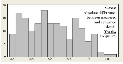
The model was tested with 230 points of known depths. The depth estimation was considered satisfactory for the test points that lied inside the zone of confidence interval of the estimated individual values (fig. 2). A number of 58 points lie outside the zone while 172, that is 75% of the total, lie inside it. The absolute differences between known depths and estimated depths at these points vary from 0.01 m to 1.52 m (fig. 3) with a mean value equal to 0.6 m and a standard deviation equal to 0.4 m. The estimated zone depths vary from 6.4m to 14.0m. The former statistical analysis indicates a very sufficient performance of the model in this area despite the absence of bands 1 and 4.
Figure 2. The graphic expression of model in area A. The red lines represent the limits of confidence interval of estimated individual values. Blue circles depict the control points and green circles depict the depth estimation points. Estimated depths are on y-axis.
Figure 3. The histogramme of absolute differences between measured and estimated depths (area A). 74% of the differences are under 1.0 m
5.1.2. Model of area B: The stepwise regression was performed for the five bands on 67 initial control points over the area. The final valid model of 45 points is given in equation (8) and its statisticparameters in table 1. This model is not satisfied by band 5 and the contribution of band 1 and 4, although statistically significant, is small.
z = 5.347 + 0.302X1 + 1.011X2–1.673X3– 0.553X4 (8)
where z = the estimated depth
X1, X2, X3, X4 = the natural logarithms of the corresponding pixel values of bands 1, 2, 3 and 4.
The model was tested with 25 points of known depths. Six points lie out of the confidence zone while 19, that is 76% of the total, lie inside it (fig. 4).The absolute differences between known depths and estimated depths at these points vary from 0.02 m to 0.36 m, (fig. 5) with a mean value equal to 0.17 m and a standard deviation equal to 0.08 m. The zone’s estimated depths vary from 2.7 m to 4.6 m. According to equation (8) more bands satisfied the model that handled very sufficiently the bottom reflectance variations.
Figure 4. The graphic expression of confidence zone in area B. The symbolisms are given in figure 2.
5.1.3. Model of area C: A strong correlation among the independent variables Xi was observed that led to a factor ana-lysis. The statistical analysis gave one factor and therefore, rather than the five image bands, the principal component (PC1)
X-axis:
Absolute differences between measured and estimated depths
Y-axis:
was used. A new simple regression analysis took place. The independent variable was the natural logarithm of the first principal component values. The regression was performed on 75 points and the final valid model of 55 points is given by equation (9):
z = -0.031 + 2.01(lnPC1) (9)
Figure 5. The histogramme of absolute differences between measured and estimated depths (area B). All of the differences are under 0.4m.
The statistical parameters of the regression models in areas A, B and C (for the parameters see Mallows, 1973, Myers, 1990, Stevens, 2002) are presented in table 1.
R R2 R2est DW VIF Rval Cp
A 0.94 0.88 0.87 1.85 <=1,7 0.954 4 B 0.97 0.93 0.93 1.82 <=3.1 0.965 5 C 0.88 0.78 0.77 1.55 --- 0.939 2
Table1. The statistical parameters
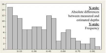
The model was tested with 178 points of known depths. The 48 of them lie outside the confidence zone while the 130 that is 73% of the total lie inside it (fig.6). The absolute differences between known depths and estimated depths at these points vary from 0.04 m to 0.93 m (fig. 7) with a mean value equal to 0.24 m and a standard deviation equal to 0.37 m. The zone’s estimated depths vary from 2.0 m to 5.8 m. According to statistical parameters and tests a very sufficient performance of the model was remarked.
Figure 6. The graphic expression of confidence zone in area C. The symbolisms are given in figure 2.
Figure 7. The histogramme of absolute differences between measured and estimated depths (area C). 67% of the differences are under 0.5m.
6. CONCLUSIONS
The linear bathymetric model was applied on the image after the sun glint removal and atmospheric correction. The image was integrated with the available echo sounding and GPS data for the calibration of the model as well as for the analysis of the corresponding depths in the area of interest. The presence of sea grass in a part of the study area and the high resolution of the image affected the linear relationship between water reflectance and depth and hindered the implementation of the model on the whole image. Thus, the water area was divided into three parts: an area with sea grass (depths about 2.0 m to 6.0 m), a mixed area with sea grass and sand (depths about 2.4 m to 6.0 m) and a sea grass-free area (depths about 6.0 m to 15.0 m). Bands 1, 2, 3, 4, and 5 of the image were used in the linear model. The outcomes of the statistical analysis indicated that the model provided very good results for the mixed and sea grass-free area, unlike the ‘sea grass’ area where the first principal component was used instead of the five image bands. In all areas the majority of the estimated depths (73-76 %), differed adequately from the soundings. The model in the mixed and the sea grass-free area was mainly influenced by the green band. The contribution of the blue band in these two areas was significant but less than the contribution of the green. The red band had a significant contribution only in the sea grass-free area that is in depths >= 6.0 m. The coastal and yellow band satisfied only the linear model of the mixed area and their contribution, although it was statistically significant, was very small. To conclude, the green band proved to be the most effective for bathymetry applications. The blue band contributed less while the red band participated only in the sea-grass free area. In general the bathymetric model involving the imagery data of high spectral and spatial resolution produced fairly accurate results. However a thorough statistical analysis was required to optimize the selection of the appropriate spectral bands.
7. REFERENCES
Andritsanos V.D., C. Pikridas, D. Rossikopoulos, I.N. Tziavos, A. Fotiou, 1997. Depth represantation in closed sea areas, la-kes and rivers using an echo sounder and the global positioning system (GPS). In Proccedings of the 4th National Carto-graphic Conference: Cartography and Maps for Success and Environment Protection, HCS, Kastoria, Greece (in greek).
Bramante J., Raju D. K. and S.T. Min, 2010. Derivation of bathymetry from multispectral imagery in the highly turbid waters of Singapore’s south islands. A comparative study.
X-axis:
Absolute differences between measured and estimated depths
Y-axis:
Frequency
X-axis:
Absolute differences between measured and estimated depths
Y-axis:
http://dgl.us.neolane.net/res/img/ac5893d9670eb994050a72130f44f444 .pdf(4 Jan. 2012)
Conger, C. L., Hochberg, E. J., Fletcher, C. H., and M. J. Atkinson, 2006. Decorrelating remote sensing color bands from bathymetry in optically shallow waters. IEEE Trans. on Geoscience and Remote Sensing, 44, pp.1655–1660.
Edwards A.J., 2010a. Les. 5: Removing sun glint from compact airborn spectrographic imager (CASI) imagery. Bilko module 7, UNESCO. http://www.noc.soton.ac.uk/bilko/module7/m7_15.php (8 Jan. 2012)
Edwards A.J., 2010b. Les. 7: Compensating for variable water depth to improve mapping of underwater habitats. Why it is
necessary. Bilko module 7, UNESCO.
http://www.noc.soton.ac.uk/bilko/module7/m7_15.php(8 Jan. 2012)
Fotiou A. and C. Pikridas, 2006. GPS and Geodetic Applications, Ziti, Thessaloniki, Greece. (in greek)
Green E., Mumby P., Edwards A. and C. Clark, 2000. Remote Sensing handbook for Tropical Coastal Management. Coastal Management Sourcebooks series, UNESCO Pub., Chapt. 8
Hatzigaki S., Karkani Z., Matziri M., Papadopoulou M., Tsakiri-Strati M., Tziavos I.N., and E. Zidrou, 2000. Multispe-ctral Bathymetry Supported by Sounding and GPS Data.Tech. Chron. Sci.J.TCG, I, 2, pp.99-110. (in greek,/ english summary)
Hedley J.D., Harborne A.R. and P.J. Mumby, 2005. Simple and robust removal of sun glint for mapping shallow-water benthos.
Int. J. Remote Sensing, 26 (10) pp. 2107-2112.
Hochberg, E.J., Andrefouet S. and M.R. Tyler, 2003. Sea su-rface correction of high spatial resolution Ikonos images to improve bottom mapping in near-shore environments, IEEE Trans. Geoscience and Remote Sensing,41(7), pp.1724-1729.
Jupp, D. L. B., 1989. Background and extension to depth of penetration (DOP) mapping in shallow coastal waters. Procee-dings of symposium on remote sensing of coastal zone, Gold Coast, Queensland, IV 2 (1) - IV 2 (19)
Kay S., Hedley J.D. and S. Lavender, 2009. Sun glint correction of high and low spatial resolution images of aquatic scenes: a review of methods for visible and near-infrared band wavelengths. Remote Sens., 1, pp. 697-730.
Kerr, J. M., 2010. Worldview-02 offers new capabilities for the monitoring of threatened coral reefs. In N.S.U.-N.C.R. Institute,editor.
http://www.digitalglobe.com/downloads/8bc/Kerr_2010_Bathymetry_fr
om_WV2.pdf. (4 Jan. 2012)
Lafazani P., 2003. Methods of Geographical Analysis, Lecture Notes, School of Rural and Surveying Engineering, Aristotle University of Thessaloniki, Thessaloniki, Greece (in greek)
Liu S., Zang J. and Y. Ma, 2010. Bathymetric ability of Spot-5 multi spectral image in shallow coastal water. In Proccedings of the 18th International Conference on Geoinformatics: GIScience in Change, Peking University, Beijing, China.
Lyons M., Phinn S. and C. Roelfsema, 2011. Inegrating Quickbird multi-spectral satellite and field data: Mapping
ba-thymetry, Seagrass Cover, Seagrass species and change in Mo-reton bay, Australia in 2004-2007. Remote Sens., 3, pp. 42-64.
Lyzenga D., 1978. Passive remote sensing techniques for mapping water depth and bottom features. Applied Optics, 17(3), pp. 379-383.
Lyzenga D., 1981. Remote sensing of bottom reflectance and ater attenuation parameters in shallow water using aircraft and Landsat data. Int. J. Remote Sensing, 2(1), pp. 71-82.
Lyzenga D., 1985. Shallow-water bathymetry using combined lidar and passive multispectral scanner data. Int. J. Remote Sensing, 6(1), pp. 115-125.
Lyzenga D., Malinas N. and F. Tanis, 2006. Multispectral bathymetry using a simple physically based algorithm. IEEE Trans. Geoscience and Remote Sensing, 44(8), pp. 2251-2259.
Mallows C.L, 1973. Some comments on Cp. Technometrics, 15, pp.661-676.
Mishra D., Narumalani S., Lawson M. and D. Rundquist, 2004. Bathymetric mapping using IKONOS multispectral data.
GIScience and Remote sensing, 41(4), pp.301-321.
Myers R., 1990. Classical and Modern Regression with Applications.2nd ed. Boston MA:Duxbury Press.
Papadopoulou M. and M. Tsakiri-Strati, 1998. Shallow sea water bathymetry using TM multispectral data. Tech. Chron. Sci.J.TCG, I(1), pp. 87-98. (in greek, extended english summary)
Paredes J. and R. Spero, 1983. Water depth mapping from passive remote sensing data under a generalized ratio assumption. Applied Optics, 22(8), pp. 1134-1135.
Philpot, W.D., 1989. Bathymetric mapping with passive multispectral imagery. Applied Optics. 28, pp.1569–1578.
Spitzer, D., and R. W. J. Dirks, 1987. Bottom Influence on the Reflectance of the Sea. Int. J. Remote Sensing, vol.8, no.3, pp.279–290.
Stevens J., 2002. Applied Multivariate Statistics for the Social Sciences. 4th ed., LEA.
Stumpf R., Holderied K. and M. Sinclair, 2003. Determination of water depth with high-resolution satellite imagery over variable bottom types. Limnol. Oceanogr., 48, pp.547-556.
Su H., Liu H. and W. Heyman, 2008. Automated derivation for bathymetric information for multispectral satellite imagery using a non-linear inversion model. Marine Geodesy, 31, pp. 281-298.
Tziavos I.N., 1996. Hydrography and Physical Oceanography, Lecture Notes, School of Rural and Surveying Engineering, Aristotle University of Thessaloniki, Thessaloniki, Greece (in greek)
Updike, T., and C. Comp, 2010. Radiometric use of WorldView-2 Imagery. Technical Note, DigitalGlobe®, Inc.