BIOCLIME Overarching report Remote Sensing Solutions GmbH Final

(1)

integration into a forest monitoring system in South Sumatra, Indonesia. Project number: 12.9013.9-001.00

Survey of biomass, carbon stocks, biodiversity, and assessment of the historic fire

regime for integration into a forest monitoring system in the Districts Musi Rawas,

Musi Rawas Utara, Musi Banyuasin and Banyuasin, South Sumatra, Indonesia

Overarching Report Work Packages 1-4

Final Report

Prepared by:

Uwe Ballhorn, Peter Navratil, Sandra Lohberger, Matthias Stängel, Werner Wiedemann, Kristina Konecny, Florian Siegert

RSS – Remote Sensing Solutions GmbH Isarstraße 3

82065 Baierbrunn Germany

(2)

(3)

Table of Content

Executive summary 5

1. Introduction 11

2. Concept of the monitoring system 12

3. Objectives 13

3.1. Work Package 3 (WP 3): Aboveground biomass and tree community composition 13 3.2. Work Package 1 (WP 1): Historic land cover change and carbon emission baseline 14 3.3. Work Package 2 (WP 2): Forest benchmark mapping and monitoring were: 14

3.4. Work Package 4 (WP 4): Historic fire regime were: 14

4. Methodological approaches and results 15

4.1. Work Package 3 (WP 3): Aboveground biomass and tree community composition 15

4.1.1. Carbon and biodiversity plots...15

4.1.2. Aboveground biomass calculations...17

4.1.3. LiDAR data and aerial photos...20

4.1.4. LiDAR based aboveground biomass model...22

4.1.5. Determination of local aboveground biomass values...24

4.1.6. LiDAR based tree community composition model...26

4.2. Work Package 1: Historic land cover change and carbon emission baseline 29 4.2.1. Dataset...29

4.2.2. Preprocessing...30

4.2.3. Land cover...31

4.2.4. Land cover change...34

4.2.5. Deforestation rate...37

4.2.6. Carbon stock...39

4.2.7. Carbon stock change...41

4.2.8. Carbon emission baseline...44

4.3. Work Package 2: Forest benchmark mapping and monitoring 46 4.3.1. Dataset...46

4.3.3. Land cover...47

4.3.4. Land cover change...52

4.3.5. Deforestation rate...56

(4)

4.3.7. Carbon stock change...60

4.4. Work Package 4: Historic fire regime 61 4.4.1. Selection of annual mid resolution images for the years 1990 – 2014...62

4.4.3. Burned area...63

4.4.4. Pre-fire vegetation...67

4.4.5. Emissions...69

5. Conclusions and outlook 71

6. Outputs / deliverables 75

(5)

Executive summary

With the Biodiversity and Climate Change Project (BIOCLIME), Germany supports Indonesia's efforts to reduce greenhouse gas emissions from the forestry sector, to conserve forest biodiversity of High Value Forest Ecosystems, maintain their Carbon stock storage capacities and to implement sustainable forest management for the benefit of the people. Germany's immediate contribution will focus on supporting the Province of South Sumatra to develop and implement a conservation and management concept to lower emissions from its forests, contributing to the GHG emission reduction goal Indonesia has committed itself until 2020.

One of the important steps to improve land-use planning, forest management and protection of nature is to base the planning and management of natural resources on accurate, reliable and consistent geographic information. In order to generate and analyze this information, a multi-purpose monitoring system is required.

This system will provide a variety of information layers of different temporal and geographic scales:

 Information on actual land-use and the dynamics of land-use changes during the past decades is considered a key component of such a system. For South Sumatra, this data is already available from a previous assessment by the World Agroforestry Center (ICRAF).

 Accurate current information on forest types and forest status, in particular in terms of aboveground biomass, carbon stock and biodiversity, derived from a combination of remote sensing and field techniques.

 Accurate information of the historic fire regime in the study area. Fire is considered one of the key drivers shaping the landscape and influencing land cover change, biodiversity and carbon stocks. This information must be derived from historic satellite imagery.

 Indicators for biodiversity in different forest ecosystems and degradation stages.

The objective of the work conducted by Remote Sensing Solutions GmbH (RSS) was to support the goals of the BIOCLIME project by providing the required information on land use dynamics, forest types and status, biomass and biodiversity and the historic fire regime. The conducted work is based on a wide variety of remote sensing systems and analysis techniques, which were jointly implemented within the project, in order to produce a reliable information base able to fulfil the project’s and the partners’ requirements on the multi-purpose monitoring system.

This report summarizes the main objectives, methodological approaches, results and conclusions from Work Packages 1 – 4:

 Work Package 1 (WP 1): Historic land cover change and carbon emission baseline

 Work Package 2 (WP 2): Forest benchmark mapping and monitoring

 Work Package 3 (WP 3): Aboveground biomass and tree community composition modelling

 Work Package 4 (WP 4): Historic fire regime

As work package 3 contains the calculation of emission factors which are used in all other work packages, this report starts with the summary of work package 3. The main objectives of WP 3 were:

(6)

 Derive Digital Surface Models (DSM), Digital Terrain Models (DTM) and Canopy Height Models (CHM) from the airborne LiDAR data.

 Advice BIOCLIME in the collection of forest inventory data to calibrate the LiDAR derived aboveground biomass model.

 Derive an aboveground biomass model from the airborne LiDAR data (provided by the project) in combination with forest inventory data (provided by the project).

 Derive local aboveground biomass values for different vegetation classes from this LiDAR based aboveground biomass model.

 Derive a tree a community composition model of Lowland Dipterocarp Forest at various degradation stages from LiDAR data (provided by the project) in combination with tree species/genera diversity data collected in the field (provided by the project).

The results of the work package were a set of local aboveground biomass (AGB) values (Emission factors) derived from the LiDAR based aboveground biomass model for almost all identified vegetation cover classes. It was shown that aboveground biomass variability within vegetation classes can be very high (e.g. Primary Dryland Forest has a standard deviation for aboveground biomass of ±222.5 t/ha). Areas with the highest aboveground biomass (AGB) values were located within and around the Kerinci Seblat National Park.

The tree community composition modelling results indicate that the similarity in tree community composition can be predicted and monitored by means of airborne LiDAR. In addition to using airborne LiDAR data as mapping tool for aboveground biomass this data could be further developed to provide a biodiversity mapping tool, so that biodiversity assessments could be carried out simultaneously with aboveground biomass analyses (same dataset). A further advantage of the approach is that the tree community composition can be carried out without identifying individual tree crowns in remotely sensed imagery.

Work package 1 focuses on the information on actual and historic land-use in the four BIOCLIME districts and the dynamics of land use changes in the past decades. The World Agroforestry Center ICRAF produced a historic time series of Land cover and land-use maps in the framework of the project LAMA-I. This dataset is provided by ICRAF for use in the Bioclime project.

The results include a wide variety of geospatial datasets, ranging from the recoded land cover classifications, land cover change, deforestation statistics and maps, carbon stock maps and statistics, carbon stock change maps, carbon change statistics, as well as a simple way of projecting a carbon emission baseline up until 2040.

(7)

The analysis of change drivers revealed that Deforestation accounts for 63 % of all changes observed between 1990 and 2014, followed by forest degradation with 20 % and Plantation expansion on Non-forest with 12%.

Net forest loss amounted to 55 % or 865,286 ha in total over the whole observation period. Annual deforestation rates increased from 2.3 % yr-1 between 1990 and 2000 to 3.8 % yr-1 between 2005 and 2010 and then further to 4.9 % yr-1 between 2010 and 2014. This increase is due to varying but more or less constant net forest loss compared to ever decreasing forested areas.

The main driver of deforestation was found to be conversion to tree crop plantation accounting for 65 % of all deforestation. However, when observed through time, this driver lost importance since the period 2000 – 2005 with 74 % of all deforestations down to 43 %. This shows a trend in tree crop plantation development to move away from forested areas to the development of already deforested areas. Other important drivers of deforestation were “Conversion to shrub” and “Conversion to Plantation forest” accounting for approximately 10 % of all deforestation in the overall observation period.

The concept of the monitoring system consists of three components: historical, current and monitoring. This report presents the outcomes of the work package 1 “Historic land cover change and carbon emission baseline” which is part of the historic component.

This work package report focuses on the first information layer listed above, the information on actual and historic land-use in the four BIOCLIME districts and the dynamics of land use changes in the past decades. The World Agroforestry Center ICRAF produced a historic time series of Land cover and land-use maps in the framework of the project LAMA-I. This dataset is provided by ICRAF for land-use in the Bioclime project. The report summarizes the calculation of the historic land cover changes and associated carbon emissions in order to contribute to the calculation of reference emission levels (REL). The results include a wide variety of geospatial datasets, ranging from the recoded land cover classifications, land cover change, deforestation statistics and maps, carbon stock maps and statistics, carbon stock change maps, carbon change statistics, as well as a simple way of projecting a carbon emission baseline up until 2040.

(8)

dryland forest (-364,692 ha). While the former was almost extent in 2014 (only 47,206 ha of former 626,024 ha left), the latter has retained 171,254 or 32 % of the original 535,947 ha. While significant parts of these losses were in the first observation window 1990 – 2000 due to logging and consequent conversion to Secondary forest, deforestation clearly dominated over time as a driver of primary forest loss. Land cover categories which increased in size include, aside from tree crop plantation, Plantation forest (+107,682 ha), Shrub (+64,357 ha), Open land (+52,928 ha), Settlement (+37,391 ha) and Mixed dryland agriculture/ mixed garden).

The analysis of change drivers revealed that Deforestation accounts for 63 % of all changes observed between 1990 and 2014, followed by forest degradation with 20 % and Plantation expansion on Non-forest with 12%.

Net forest loss amounted to 55 % or 865,286 ha in total over the whole observation period. Annual deforestation rates increased from 2.3 % yr-1 between 1990 and 2000 to 3.8 % yr-1 between 2005 and 2010 and then further to 4.9 % yr-1 between 2010 and 2014. This increase is due to varying but more or less constant net forest loss compared to ever decreasing forested areas.

The main driver of deforestation was found to be conversion to tree crop plantation accounting for 65 % of all deforestation. However, when observed through time, this driver lost importance since the period 2000 – 2005 with 74 % of all deforeations down to 43 %. This shows a trend in tree crop plantation development to move away from forested areas to the development of already deforested areas. Other important drivers of deforestation were “Conversion to shrub” and “Conversion to Plantation forest” accounting for approximately 10 % of all deforestation in the overall observation period.

The analysis of carbon stock distribution over time shows the highest carbon storage was and is found in primary dryland forest with 50,177,548 t C in 2014. However, the second highest carbon stocks are found in the tree crop plantation class which accounts for 35,800,171 t C in 2014 due to its dominant spatial extent in the AOI. Secondary dryland forest with 20,816,296 t C has the next highest carbon stocks followed by Primary Mangrove Forest with 16,001,771 t C.

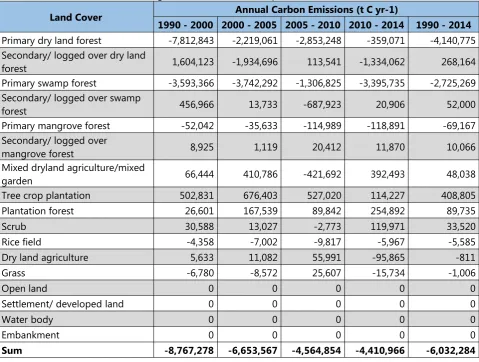
The most intensive carbon losses were observed in the class Primary dryland forest, amounting to -106,854,800 t C followed by primary peat swamp forest with -80,745,135 t C. These intense losses were only partly compensated by carbon accumulation in Tree crop plantations amounting to 15,023,600 t C and Plantation forest (3,445,819 t C). Annual total carbon losses amounted totaled at -9,360,247 t C yr-1 in the period yr-1990-2000, constantly declining to -5,yr-128,6yr-14 t C yr-yr-1 in the period 20yr-10 – 20yr-14. The overall average 1990 – 2014 was -6,611,873 t C yr-1

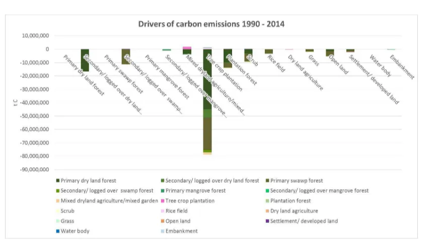
The analysis of the drivers of carbon emissions showed that the main process causing emissions is the conversion into tree crop plantations which account for over 80,000,000 t C in the observation period 1990 – 2014. The majority of those emissions came from the conversion of Primary dryland forest, followed by Primary swamp forest. The second highest emissions were caused from logging of Primary dryland forest, accounting for approximately 16,000,000 t C followed by the conversion to Plantation forest which produced another 15,000,000 t C. Logging of primary swamp forest caused another 12,000,000 t C.

(9)

approximately 100,000,000 t C which means the predicted emissions under a business as usual scenario amount to approximately 50,000,000 t C in the next 25 years, i.e. approximately 2,000,000 t C yr-1 as a long term annual average.

The key objective of work package 2 was the processing of high resolution satellite images in order to create a forest benchmark map for the project areas KPHP Benakat, KPHK Bentayan, Dangku Wildlife Reserve, Kerinci Seblat National Park, KPHP Lakitan, KPHP Lalan, Mangrove, PT Reki and Sembilang National Park, including information on forest carbon stock, forest types, deforestation and in particular forest degradation. The first update of the map was done in 2016 based on newly acquired data in order to assess/monitor the changes of forest carbon stocks for the years 2014 to 2016 under project conditions.

The benchmark land cover maps produced have a high overall thematic accuracy (84.4 % according to the BAPLAN classification scheme) which makes them an ideal basis for future monitoring. The most recent classification was completed in 2016 and was based on RapidEye imagery. Kerinci Seblat National Park is the only region where RapidEye coverage was incomplete and a filling with Landsat-8 imagery was required. The way the classification algorithm was designed allowed an easy transfer and application to the images from the second time step and also enabled the maps from the second time step to achieve an overall accuracy of 87%.

A combination of these land cover maps, forest inventory and relevant LiDAR based AGB modeling provided information on forest carbon stocks. This data showed a decrease in carbon stocks across each AOI during the study period.

The lowest decreases in carbon stock per hectare was found in Kerinci Seblat National Park and KPHP Benakat (1%). Medium-density lowland dipterocarp forest in Kerinci Seblat National Park lost the most carbon (194,820 t) of all forest classes, experiencing a deforestation rate of just 0.8%. Meanwhile, KPHP Benakat experienced a relatively high deforestation rate of 4.5% proportional to its decrease in carbon stock. In Benakat, forest loss of low-density lowland dipterocarp forest had the largest impact, removing 38,104 tons of carbon.

KPHP Bentayan experienced a reduction of average carbon stock per hectare by around 6%, documenting a deforestation rate of 5.4%. Furthermore, although carbon losses in non-forest classes were greater than those in forest classes, net forest loss still amounted to 1,196 ha in Bentayan.

Dangku Wildlife Reserve experienced immense carbon stock losses within medium-density lowland dipterocarp forests (315,051 t). These led to a 6% reduction in average carbon stock per hectare, a net forest loss of 759 hectares and finally, a deforestation rate of 1.5%.

(10)

The second largest reduction in average carbon stock amounted to 11% and was found in KPHP Lakitan. Within Lakitan, medium-density lowland dipterocarp forest lost approximately 0.6 million tons, the net forest loss amounted to 3,717 hectares and a deforestation rate of 10.4% was recorded.

The highest reduction of average carbon stock was by far was recorded in KPHP Lalan at 53%. In this region, high-density peat swamp forest alone lost nearly four million tons of carbon. This contributed to a deforestation rate of 36.3% and a net forest loss of 53,176 ha.

The key objective of work package 4 was the generation of burned area maps for different years based on optical satellite data. The years for classification were selected based on the numbers of hotspots (MODIS) per year and precipitation distributions. Only the burned areas for severe fire years were classified (1997, 1999, 2002, 2004, 2006, 2009, 2011, 2012, 2014 and 2015). Historic satellite data (Landsat-5, Landsat-7 and Landsat-8) was utilized from the period 1997 onwards to assess the historic fire regime. Burned areas were classified based on the combination of two methodologies to increase accuracy. The result of the classification is a yearly map of burned areas within the boundaries of the BIOCLIME study area. Based on these maps a fire frequency map was derived in order to locate areas of higher and lower fire frequency. Based on these annual burned areas emissions were calculated to assess the amount of carbon emitted, from the vegetation cover and the peat soil. The results are annual and total emissions from aboveground biomass, peat burning within the BIOCLIME study area. The results of the work package show that while a direct deduction of burned area from the amount of fire hotspots is feasible, it should always be treated with caution and only general trends can be derived. The spatially explicit assessment conducted in this work package based on Landsat data showed reliably that in 1997 the share of burned Primary Forest is by far the biggest. The second largest Primary Forest burning took place in 2006. The burning of the land cover classes Tree Crop Plantation and Plantation Forest is increasing over the years. There is a clear change in ratio of land cover classes burned over the last two decades.

(11)

1. Introduction

This system will provide a variety of information layers of different temporal and geographic scales:

 Information on actual land-use and the dynamics of land-use changes during the past decades is considered a key component of such a system. For South Sumatra, this data is already available from a previous assessment by the World Agroforestry Center (ICRAF).

 Accurate current information on forest types and forest status, in particular in terms of aboveground biomass, carbon stock and biodiversity, derived from a combination of remote sensing and field techniques.

 Accurate information of the historic fire regime in the study area. Fire is considered one of the key drivers shaping the landscape and influencing land cover change, biodiversity and carbon stocks. This information must be derived from historic satellite imagery.

 Indicators for biodiversity in different forest ecosystems and degradation stages.

The objective of the work conducted by Remote Sensing Solutions GmbH (RSS) was to support the goals of the BIOCLIME project by providing the required information on land use dynamics, forest types and status, biomass and biodiversity and the historic fire regime. The conducted work is based on a wide variety of remote sensing systems and analysis techniques, which were jointly implemented within the project, in order to produce a reliable information base able to fulfil the project’s and the partners’ requirements on the multi-purpose monitoring system.

This report summarizes the main objectives, methodological approaches, results and conclusions from Work Packages 1 – 4:

 Work Package 1 (WP 1): Historic land cover change and carbon emission baseline  Work Package 2 (WP 2): Forest benchmark mapping and monitoring

 Work Package 3 (WP 3): Aboveground biomass and tree community composition modelling

 Work Package 4 (WP 4): Historic fire regime

(12)

Figure 1: The BIOCLIME districts and the nine project areas.

2. Concept of the monitoring system

The four Work Packages mentioned above form the basis of the developed monitoring system. The concept of the monitoring system consists of three components: historical, current and monitoring (Figure 2). The historical component includes an analysis of the historic fire regime on the basis of Landsat imagery (WP 4: Historic fire regime) as well as historic land cover change maps produced by ICRAF (international Center for Research in Agroforestry) in order to identify drivers of deforestation and carbon emissions (WP 1: Historic land cover change and carbon emission baseline). The current component comprises the development the development of aboveground biomass and tree community composition models from airborne LiDAR data (WP 3: Aboveground biomass and tree community composition modelling) as well as a forest benchmark map derived from high resolution satellite images (WP 2: Forest benchmark mapping and monitoring) in order to create and retrieve local aboveground biomass values (WP 3: Aboveground biomass and tree community composition modelling). The main objectives, methodological approaches, results and conclusions for each of the Work Packages is described in the following text. A more detailed description of these Work Packages is given the respective Work Package final reports.

(13)

Figure 2: Concept of the monitoring system. Also shown is which parts of the monitoring system are covered by which Work Packages: WP 1 (Work Package 1): Historic land cover change and carbon emission baseline; WP 2 (Work Package 2): Forest benchmark mapping and monitoring; WP 3 (Work Package 3: Aboveground biomass and tree community composition modelling; WP 4 (Work Package 4): Historic fire regime.

3. Objectives

3.1. Work Package 3 (WP 3): Aboveground biomass and tree community

composition

 Filtering of the LiDAR 3D point clouds (provided by the project) into vegetation and non-vegetation points.

 Derive Digital Surface Models (DSM), Digital Terrain Models (DTM) and Canopy Height Models (CHM) from the airborne LiDAR data.

 Advice BIOCLIME in the collection of forest inventory data to calibrate the LiDAR derived aboveground biomass model.

 Derive an aboveground biomass model from the airborne LiDAR data (provided by the project) in combination with forest inventory data (provided by the project).

 Deduce local aboveground biomass values for different vegetation classes from this LiDAR based aboveground biomass model.

 Derive a tree a community composition model of Lowland Dipterocarp Forest at various

(14)

3.2. Work Package 1 (WP 1): Historic land cover change and carbon emission

baseline

 Assessment of the historic land cover (1990, 2000, 2005, 2010 and 2014) in the four BIOCLIME districts based on a historic land cover data set (Version 3) provided by the World Agroforestry Center (ICRFA).

 Derivation and assessment of the historic land cover change and dynamics based on this dataset.

 Derivation and assessment of the historic carbon stocks based on this data set and local aboveground biomass values derived in Work Package 3 (WP 3):

Aboveground biomass and

tree community composition modelling.

 Derivation and assessment of the carbon stock changes derived from these carbon stock estimates in order to contribute to the calculation of the reference emission level (REL).



Derivation of an emission baseline in order to contribute to the calculation of the reference emission level (REL).

3.3. Work Package 2 (WP 2): Forest benchmark mapping and monitoring were:

 Preprocessing of high resolution satellite images (SPOT and RapidEye) for the project areas KPHP Benakat, KPHP Bentayan, Dangku Wildlife Reserve, Kerinci Seblat National Park, KPHP Lakitan, KPHP Lalan, Mangrove, PT Reki and Sembilang National Park for the years 2014 and 2016.

 Derivation and assessment of the land cover for 2014 (forest benchmark) and 2016 (monitoring) based on these high resolution satellite images.

 Derivation and assessment of the land cover change and dynamics between 2014 and 2016.

 Derivation and assessment of the carbon stocks based on the above derived land cover and the local aboveground biomass values from Work Package 3 (WP 3): Aboveground biomass and tree community composition modelling.

 Derivation and assessment of the carbon stock changes derived from these carbon stock

estimates.

3.4. Work Package 4 (WP 4): Historic fire regime were:

 Selection of annual mid resolution satellite images (Landsat) for the fire years 1990-2014

covering the four BIOCLIME districts.

 Preprocessing of these mid resolution satellite images (Landsat).

 Derivation and assessment burned areas for these fire years based on these mid resolution satellite images (Landsat).

(15)

from Work Package 3 (WP 3): Aboveground biomass and tree community composition modelling.

 Derivation and assessment of the peat fire emissions based on these yearly classified burned areas, a peatland distribution map provided by the Ministry of Environment and Forestry (MoEF), the historical land covers derived in Work Package 1 (WP 1): Historic land cover change and carbon emission baseline and peat burned depths based on a publication by Konecnyet al.(2015).

4. Methodological approaches and results

4.1. Work Package 3 (WP 3): Aboveground biomass and tree community

composition

Figure 2 shows the flowchart of the activities carried out in Work Package 3 (WP 3): Aboveground biomass and tree community composition modelling.

Figure 2: Flow chart of the activities carried out in Work Package 3 (WP 3): Aboveground biomass and tree community composition modelling.

4.1.1.Carbon and biodiversity plots

(16)

Bogor Agricultural University (IPB) and BIOCLIME. The distribution of these carbon inventory plots is based on a systematic sampling design. In order, to assure that statistically enough carbon inventory plots are located within the airborne LiDAR transects to generate the LiDAR based aboveground biomass model some of these 112 plots where spatially shifted into the nearest LiDAR transect, consequently now not fitting into the systematic sampling design anymore. In natural forests a nested rectangular plot design was chosen (0.1 ha) and in plantations a circular plot design was applied, where the size of the circle depended on the age of the plantation (age of plantation < four years: radius = 7.98 m, area = 0.02 ha; age of plantation ≥ four years: radius = 11.29 m, area = 0.04 ha). For all “in” trees (an “in” tree was defined as a tree where the center of the stem at DBH was within the boundaries of the respective (sub)plot) Diameter at Breast Height (DBH; in centimeter), total tree height (in meter), trees species (scientific name in Latin) and four dead wood classes were recorded. Additionally, to the carbon plots 58 so called biodiversity plots were recorded. The spatial locations of these biodiversity plots are exactly the same as the ones of the respective carbon plot. For all “in” trees within the biodiversity plots Diameter at Breast Height (DBH; in centimeter) and tree species (scientific name in Latin) were recorded.

Table 1 gives an overview on how many carbon and biodiversity plots were recorded and whether they are located within LiDAR transects or not. As can be seen in Table 1, six plots were recorded after the fires of 2015. These plots have to be treated with care, as the LiDAR data was recorded before the fires of 2015.

Table 1: Overview carbon and biodiversity plots recorded and whether they are located within LiDAR transects or not.

Carbon plots Biodiversity plots Amount plots Amount plots withinLiDAR transects

X 54 (521₎ _{15 (13}1₎

X X 58 (551₎ _{48 (45}1₎

Sum 112 (1071₎ _{63 (68}1₎

1_{Amount of plots after subtracting plots that were recorded after the fires of 2015}

(17)

4.1.2.Aboveground biomass calculations

Rusolono et al. (2015) provide detailed procedures for analyzing the carbon stocks of the five carbon pools: aboveground biomass (AGB), belowground biomass (BGB), dead-wood, litter and soils. As the derived LiDAR AGB model is based on the estimated AGB from the carbon inventory plots only the derivation of AGB will be described in this report.

(18)

Manuri et al. (2014) and Komiyamaet al. (2005) were used to estimate tree AGB for dryland forests, peat swamp forests and other mangrove species (i.e. Excoecaria agallocha and Sonneratia caseolaris), respectively.

Table 3: Allometric biomass models for estimating tree aboveground biomass (AGB).

Tree species Allometric model Statistics Location Source

Plantation forest

Acacia mangium Wag= 0.070*D2.580 D: 8–28 cm

R2_{= 0.97}

South Sumatra Wicaksono (2004) cited in Krisnawatiet al.(2012)

Eucalyptus pellita1 _W_ag_{= 0.0678*D}2.790 _D_{: 2–27 cm}

R2_{= 0.99}

South Sumatra Onrizal et al. (2009) cited in Krisnawatiet al.(2012)

Estate crop

Hevea brasiliensis Wag= 0.2661*D2.1430 Elias (2014)

Elaeis guineensis Wag= 0.0706 + 0.0976*H Sumatra, Kalimantan ICRAF (2009) cited in

Hairiahet al.(2011)

Dryland forest

Tropical mixed species Wag= 0.0673 (p*D2*H)0.976 D: 2–212 cm Africa, America, Asia Chaveet al.(2014)

Peat swamp forest

Mixed species Wag= 0.15 D2.0.95*p0.664*H05526 D: 2–167 cm

R2_{= 0.981}

Riau, South Sumatra,

West Kalimantan Manuriet al.(2014)

Mangrove forest Avicennia marina, Avicennia alba1

Wag= 0.1846*D2.352 D: 6–35 cm

R2_{= 0.98}

West Java Darmawan & Siregar (2008) cited in Krisnawatiet al.(2012)

Bruguiera gymnorrhiza Wag= 0.1858*D2.3055 D: 2–24 cm

R2_{= 0.989}

Australia Clough & Scott (1989)

Bruguiera parviflora, Bruguiera sexangula1

Wag= 0.1799*D2.4167 D: 2–21 cm

R2_{= 0.993}

Ceriops tagal Wag= 0.1884*D2.3379 D: 2–18 cm

R2_{= 0.989}

Rhizophora apiculate, Rhizophora mucronata1

Wag= 0.235*D2.42 D: 5–28 cm

R2_{= 0.98}

Malaysia Onget al.(2004)

Xylocarpus granatum Wag= 0.0823*D2.5883 D: 3–17 cm

R2_{= 0.994}

Other species (Excoecaria agallocha,

Sonneratia caseolaris)

Wag= 0.2512*p*D2.46 D: 5–49 cm

R2_{= 0.979}

Indonesia, Thailand Komiyamaet al.(2005)

Wag= aboveground biomass (kg),D= Diameter at Breast Height (DBH, cm),H= tree height (m),p= wood density (gram/cm3),R2=

coefficient of determination

1_{The aboveground biomass of these tree species were estimated using the available allometric models for similar tree species.}

(19)

of the total tree species), the allometric models used average wood density values that were derived from identified tree species in a particular stratum and location (Table 5).

Table 4: Diameter-height models for estimating tree height in some surveyed areas.

Stratum1 Location Model Statistics

Secondary / Logged over Dryland Forest (Hutan Lahan Kering Sekunder / Bekas Tebangan)

PT REKI H=D/(0.7707+0.0195*D) nAIC= 168,= 1032.21,D= 5–104 cm,RMSE= 5.58,

R2_adj_{= 0.624}

BKSDA Dangku H= exp(0.7071+0.6556*ln(D)) nAIC= 156,= 845.56,D= 6–69 cm,RMSE= 3.75,

R2

adj= 0.690

Primary Mangrove Forest

(Hutan Mangrove Primer) TN Sembilang H= 28.1613*(1-exp(-D/27.0703))

n= 221,D= 5-77 cm,

AIC= 1098.86,RMSE= 2.89,

R2_adj_{= 0.750}

D= Diameter at Breast Height (DBH, cm),H= tree height (m),n= number of samples,AIC= Akaike Information Criterion,RMSE= root mean square error,R2_adj_{= coefficient of determination adjusted}

1_{in brackets Bahasa Indonesia}

Table 5: Average wood density for unidentified tree species.

Startum1 Location Mean

(g/cm3₎ _(g/cmSt.dev.3₎2

Primary Dryland Forest

(Hutan Lahan Kering Primer) TN Kerinci Seblat 0.615 0.142 Secondary / Logged over Dryland Forest

(Hutan Lahan Kering Sekunder / Bekas Tebangan) PT REKI 0.594 0.143 Primary Mangrove Forest

(Hutan Mangrove Primer) Banyuasin 0.702 0.077 Secondary / Logged over Swamp Forest

(Hutan Rawa Sekunder / Bekas Tebangan) TN Sembilang 0.643 0.115 1_{in brackets Bahasa Indonesia}

2_{standard deviation}

Some carbon inventory plots (i.e. 7 plots or 4.9% of the total sample plots) also contained non-woody vegetation (i.e. bamboo, palm or rattan). The quantity of such non-woody vegetation, however, was very low with incomplete measurements of diameter or height, which resulted in difficulties when estimating their biomass. Therefore, the quantification of this insignificant non-woody biomass for these 7 sample plots was ignored.

The biomass of understory vegetation in each carbon inventory plot was estimated based on the field measurements and a laboratory analysis of the understory vegetation samples. The field measurements provided data on the sample’s fresh weight and total fresh weight of the understory vegetation, while the laboratory analysis provided data on the sample’s dry weight of the understory vegetation. The aboveground biomass of the understory vegetation was then calculated on the ratio of dry and fresh weights of the sample, which was then multiplied with the total fresh weight of the understory vegetation within a sample plot.

(20)

biomass for each sample plot. Aboveground biomass estimates per plot in tons per hectare (t/ha) for the carbon plots are shown in Appendix A. Table 6 summarizes the aboveground biomass estimates for the different strata. An in-depth explanation of the results and methods applied in the field inventory is provided in the BIOCLIME GIZ Final Report: Cadangan Karbon Hutan dan Keanekaragaman Flora di Sumatera Selatan (Tiryanaet al.2015).

Table 6: Statistical results for the aboveground biomass (AGB) estimates for the different strata. Stratum1 Number of carbon

inventory plots

Min AGB

(t/ha)2 Max AGB_(t/ha)3 Mean AGB_(t/ha)4

Primary Dryland Forest

(Hutan Lahan Kering Primer) 8 196.1 637.0 335.6 ±153.8 Secondary / Logged over Dryland Forest

(Hutan Lahan Kering Sekunder) 33 69.1 560.7 259.0 ±129.0 Primary Mangrove Forest

(Hutan Mangrove Primer) 13 159.8 531.3 304.7 ±98.8 Secondary / Logged over Mangrove Forest

(Hutan Mangrove Sekunder) 7 44.9 342.5 174.0 ±114.1 Primary Peat Swamp Forest

(Hutan Rawa Gambut Primer) 5 442.4 616.0 538.1 ±64.9 Secondary / Logged over Peat Swamp

Forest

(Hutan Rawa Gambut Sekunder) 9 114.9 414.0 207.1 ±89.9 Plantation Forest

(Hutan Tanaman) 8 5.4 133.8 59.9 ±43.7

Tree Crop Plantation

(Perkebunan) 15 3.4 211.6 62.2 ±55.4

Shrubs

(Semak Belukar) 6 8.7 127.2 59.6 ±54.0

Swamp Shrubs

(Semak Belukar Rawa) 8 1.3 105.5 55.5 ±41.5

Sum 112

1_{in brackets Bahasa Indonesia}

2_{Minimum aboveground biomass (AGB) in tons per hectare for the stratum} 3_{Maximum aboveground biomass (AGB) in tons per hectare for the stratum}

4_{Mean aboveground biomass (AGB) in tons per hectare for the Stratum class (± = standard deviation)}

4.1.3.LiDAR data and aerial photos

In October 2014 15 transects of LiDAR data and aerial photos were captured for an area of approximately 43,300 ha. LiDAR data was acquired in two modes (a) LiDAR full waveform mode + aerial photos with an overlap of 60% and (b) LiDAR discrete return mode + aerial photo overlap 80%. Figure 4 shows the location of the LiDAR transects within the BIOCLIME study area.

(21)

Figure 5: Example of LiDAR 3D point clouds for Lowland Dipterocarp Forest, Peat Swamp Forest and Mangrove.

(22)

Figure 6: Example from the LiDAR products generated for the BIOCLIME study area. Shown are examples for the Digital Terrain Model (DTM; 1 m spatial resolution) the Digital Surface Model (DSM; 1 m spatial resolution) and the Canopy Height Model (CHM; 1 m spatial resolution). Also shown are the position of the 66 carbon plots that are located within the LiDAR transects.

4.1.4.LiDAR based aboveground biomass model

Previous studies revealed that height metrics like the Quadratic Mean Canopy Height (QMCH) or the Centroid Height (CH) are appropriate parameters of the LiDAR 3D point cloud to estimate aboveground biomass in tropical forests (Jubanskiet al.2013, Englhartet al.2013, Ballhornet al.2011). The commonly used power function resulted in significant overestimations in the higher biomass range within our study areas. For this reason, a more appropriate aboveground regression model was implemented, which is a combination of a power function (in the lower biomass range up to a certain threshold QMCH0; the example here uses QMCH but the same would be done with CH) and a linear function (in the higher biomass range) (Englhartet al.2013).

(23)

model. The LiDAR based aboveground biomass model was created at 5 m spatial resolution i.e. each pixel represents an area of 0.1 ha. For ease of interpretation the cell values were scaled to represent aboveground biomass in tons per hectare. Figure 7 displays the final LiDAR based aboveground biomass model and gives examples of Lowland Dipterocarp Forest, Peat Swamp Forest and Mangrove.

(24)

4.1.5.Determination of local aboveground biomass values

In order to derive local aboveground biomass values for the different land cover classes, the spatial aboveground biomass model was overlaid with the land cover classification from Work Package 2 (WP 2) and zonal statistics (minimum, maximum, mean and standard deviation) on aboveground biomass were extracted for the respective land cover class.

Zonal statistics were extracted for the BAPLAN and BAPLAN enhanced land cover classes. Table 4 and Table 5 display these derived local aboveground biomass values. For the land cover classes not present in the aboveground biomass model missing values were estimated based on existing values or missing values were based on values from scientific literature.

These local aboveground biomass values were used for the emission calculations in the other work packages (WP 1, WP 2 and WP 4).

Table 4: Local aboveground biomass values derived from zonal statistics of the LiDAR aboveground biomass model for the different forest type / land cover classes based on BAPLAN.

Forest type / land cover BAPLAN1 Mean AGB (t/ha)2 SD (t/ha)3 Min AGB (t/ha)4 Max AGB (t/ha)5 Area (ha)6

Primary Dryland Forest 586 ±157.8 38.2 1,404.8 2,285.2 Secondary / Logged over Dryland Forest 305 ±158.8 0.0 1,206.5 5,685.3

Primary Swamp Forest 279 ±97.8 4.7 709.0 1,806.5

Secondary / Logged over Swamp Forest 108 ±78.6 0.2 505.4 1,363.3

Primary Mangrove Forest 249 ±106.7 0.0 668.8 4,031.9

Secondary / Logged over Mangrove Forest 72 ±34.4 14.0 284.4 71.7 Mixed Dryland Agriculture / Mixed Garden 144 ±100.2 0.0 712.3 1,883.0

Tree Crop Plantation 49 ±63.2 0.0 428.9 442.2

Plantation Forest 64 ±45.8 0.0 406.5 517.5

Scrub 39 ±57.3 0.0 762.4 964.6

Swamp Scrub 15 ±19.1 0.2 123.1 3.3

Rice Field7 ₁₀ _- _- _-

-Dryland Agriculture 48 ±64.1 0.0 487.0 126.3

Grass8 ₆ _- _- _-

-Open Land9 _{(0) 29} _±75.7 _0.0 _749.0 _13.4

Settlement / Developed Land9 _{(0) 23} _±14.8 _0.2 _81.8 _1.3

Water Body9 _{(0) 164} _±68.8 _1.1 _469.3 _83.2

Swamp 22 ±20.7 0.3 80.8 1.3

Embankment9 _{(0) 2} _±4.1 _0.0 _25.1 _9.5

1_{Forest type/land cover class BAPLAN classification system}

2_{Mean aboveground biomass (AGB) in tons per hectare for the forest type/land cover class} 3_{Standard deviation (SD) in tons per hectare for the forest type/land cover class}

4_{Minimum aboveground biomass (AGB) in tons per hectare for the forest type/land cover class} 5_{Maximum aboveground biomass (AGB) in tons per hectare for the forest type/land cover class} 6_{Area in hectare from which zonal statistics are based on}

7_{Value for Rice Field from scientific literature (Confalonieri}_{et al.}₂₀₀₉₎ 8_{Value for Grass from scientific literature (IPCC 2006)}

(25)

Table 5: Local aboveground biomass values derived from zonal statistics of the LiDAR aboveground biomass model for the different forest type / land cover classes based on BAPLAN enhanced.

Forest type / land cover BAPLAN enhanced1 Mean AGB

(t/ha)2 SD (t/ha)3 Min AGB_(t/ha)4 Max AGB_(t/ha)5 Area (ha)6

High-density Upper Montane Forest7 ₃₀₄ _- _- _-

-Medium-density Upper Montane Forest8 ₂₂₈ _- _- _-

-Low-density Upper Montane Forest7 ₁₉₂ _- _- _-

-High-density Lower Montane Forest 653 ±129.0 229.6 1106.7 52.0

Medium-density Lower Montane Forest 529 ±77.3 358.3 789.0 5.5

Low-density Lower Montane Forest7 ₂₆₈ _- _- _-

-High-density Lowland Dipterocarp Forest 584 ±158.0 38.2 1404.8 2,233.2

Medium-density Lowland Dipterocarp Forest 340 ±152.7 0.0 1206.5 4,536.6

Low-density Lowland Dipterocarp Forest 166 ±92.8 0.3 986.8 1,143.2

High-density Peat Swamp Forest 287 ±100.0 5.3 709.0 1,430.7

Medium-density Peat Swamp Forest8 ₂₁₆ _- _- _-

-Low-density (Regrowing) Peat Swamp Forest 110 ±86.6 0.9 505.4 590.7

Permanently Inundated Peat Swamp Forest 244 ±86.9 4.7 568.1 301.1

High-density Swamp Forest

(incl. Back- and Freshwater Swamp) 256 ±52.5 13.5 399.0 74.8

Medium-density Swamp Forest

(incl. Back- and Freshwater Swamp)8 192 - - -

-Low-density (Regrowing) Swamp Forest

(incl. Back- and Freshwater Swamp) 107 ±71.9 0.2 444.4 772.6

Heath Forest7 ₂₂₄ _- _- _-

-Mangrove 1 268 ±99.8 0.0 668.8 3,473.1

Mangrove 2 200 ±95.7 26.2 515.3 86.0

Nipah Palm 115 ±37.8 0.9 456.6 472.8

Degraded Mangrove 74 ±34.9 14.0 218.9 57.8

Young Mangrove 65 ±31.0 17.5 284.4 13.9

Dryland Agriculture mixed with Scrub 38 ±47.1 0.0 508.8 414.2

Rubber Agroforestry 174 ±90.4 0.0 712.3 1,468.8

Oil Palm Plantation 27 ±42.2 0.0 336.0 304.2

Coconut Plantation 58 ±27.1 2.5 132.2 94.1

Rubber Plantation 185 ±66.6 0.6 428.9 43.9

Acacia Plantation 64 ±48.6 0.0 236.6 360.2

Industrial Forest 63 ±38.7 0.5 406.5 157.3

Scrubland 39 ±57.3 0.0 762.4 964.6

Swamp Scrub 15 ±19.1 0.2 123.1 3.3

Rice Field9 ₁₀ _- _- _-

-Dryland Agriculture 48 ±64.1 0.0 487.0 126.3

Grassland10 ₆ _- _- _-

-Bare Area11 _{(0) 29} _±75.7 _0.0 _749.0 _13.4

Settlement11 _{(0) 10} _±14.2 _0.2 _81.8 _0.4

Road11 _{(0) 29} _±10.6 _0.3 _49.6 _0.9

Water11 _{(0) 164} _±68.8 _1.1 _469.3 _83.2

Wetland 22 ±20.7 0.3 80.8 1.3

Aquaculture11 _{(0) 2} _±4.1 _0.0 _25.1 _9.5

1_{Forest type/land cover class BAPLAN enhanced classification system} 7_{Values from FORCLIME (Navratil 2012)} 2_{Mean aboveground biomass (AGB) in tons per hectare for the forest type/land cover class} 8_{Calculated as 75% of respective high density class}

3_{Standard deviation (SD) in tons per hectare for the forest type/land cover class} 9_{Value for Rice Field from scientific literature (Confalonieri}_{et al.}₂₀₀₉₎ 4_{Minimum aboveground biomass (AGB) in tons per hectare for the forest type/land cover class} 10_{Value for Grass from scientific literature (IPCC 2006)}

5_{Maximum aboveground biomass (AGB) in tons per hectare for the forest type/land cover class} 11_{Value in brackets was finally used as local aboveground biomass value as}

the

(26)

4.1.6.LiDAR based tree community composition model

Within all the biodiversity plots 378 types of species where identified belonging to 192 genera. Table 6 displays the absolute numbers and percentage of trees within the biodiversity plots where the species could be identified, where only genus, family, common name was known and unidentified trees.

Table 6: Absolute and percentage of tree identification (species, only genus, only family, only common name and unidentified) within the biodiversity plots.

All trees

recorded identifiedSpecies Only genusidentified Only familyidentified Only commonname Unidentified Absolute

number 2733 2408 284 15 4 22

Percent (%) 100% 88% 10% 1% 0% 1%

All further analyses on tree community composition were conducted for lowland dipterocarp forest only. Mangrove was excluded as the variety of different tree species in the observed mangroves was very low (only up to six different tree species). Peat swamp forest was excluded because only three biodiversity plots were available and all were recorded after the fires of 2015.

Because some trees could not be identified to the species level all analyses on tree community composition are based on the genus level. Imaiat al.(2014) showed that results on the genus level are highly correlated with those at the species level.

To assess the effects of different degradation levels on forest biodiversity the degree of similarity in tree community composition has gained increasing attention (Lokiet al. 2016, Barlowet al. 2007, Imai et al. 2012, Imai et al. 2014, Magurran and McGill 2011, Su et al. 2004, Ding et al. 2012). Nonmetric multidimensional scaling (nMDS) was applied to assess the differences in tree community composition among the biodiversity plots. The number of trees of each genus within the 38 biodiversity plots located in lowland dipterocarp forest was used as input to the Bray-Curtis similarity index to calculate the nMDS scores of axis 1 and axis 2. As there was no statistical significant correlation between forest density classes (Low-, Medium- and High-density Lowland Dipterocarp Forest) and the nMDS scores of axis 2, only scores from axis 1 very implemented in subsequent analyses. Further five biodiversity indices were calculated per biodiversity plot (Simpson index 1-D, Shannon index (entropy), Margalef’s richness index, Equitability, Ratio pioneer/climax tree species).

(27)

Lowland Dipterocarp Forest feature proportionally more pioneer tree species and vice versa. All these findings indicate that high nMDS axis 1 scores go hand in hand with higher ‘richness/diversity’ and ‘evenness’ and that the occurrence of climax tree species in comparison to pioneer tree species is favored.

Next, to test whether there is a statistical significant difference between the different density classes (density stratification based on forest cover at 10 m height) with regard to nMDS and the biodiversity indicators a One-way ANOVA was performed. When the ANOVA results were significant, a Tukey’s pairwise post-hoc test was used to identify the different pairs of groups. Results showed that there was a statistical significant (p< 0.05) difference between the means of the different density classes (Low, Medium and High) for the nMDS axis 1 scores, Shannon index and Margelef’s index. Further, for all these three indicators the Tukey’s pairwise post-hoc test showed there was a statistical significant (p< 0.05) difference between the density pairs Low vs Medium and Low vs High but not for Medium vs High. These statistical results indicate that there is a significant different with regard to tree community composition between these different density classes and that the density classes Low vs Medium and Low vs High could be best differentiated.

From the airborne LiDAR data 19 LiDAR metrics per biomass plot located within a LiDAR transect (n = 28) were derived. These LiDAR metrics were then correlated to the nMDS scores of axis 1 in order to derive a predictive LiDAR based tree community composition model. A stepwise forward and backward multiple regression was performed (R software was used for this). The final model included three significant variables (Mean, cov 12m = forest cover in percent at 12 m height and p 50th _{= 50}th percentile) and four biodiversity plots were excluded (outliers) from the model development. Anr2_of

0.72 was obtained (n = 24).

(28)

(29)

4.2. Work Package 1: Historic land cover change and carbon emission baseline

Figure 9 shows the flowchart of the activities carried out in Work Package 1 (WP 1): Historic land cover change and carbon emission baseline.

Figure 9: Flow chart of the activities carried out in Work Package 1 (WP 1): Historic land cover and carbon emission baseline.

4.2.1.Dataset

(30)

Table 7: Datasets provided by ICRAF

Filename Type Format

LC1990_v3_48s.tif Raster GeoTIFF

GPS_accuracy_all.shp Point Vector Shapefile

lc_legend.lyr Symbology Layerfile

lc_legend.xlsx Spreadsheet MS Excel

Accuracy_Assessment_result.docx Report MS Word

Technical report_LAMA-I_TZ_AP_VA_18062015.pdf Report PDF

A detailed technical assessment of the Version 2 of the data was conducted and the results are summarized in the internal report “Quality assessment report of ICRAF historic land cover change dataset”. The report proved a very high quality of the analysis conducted, however, identified a variety of shortcomings of Version 2. As a consequence, a follow up Version 3 of the data was produced by ICRAF, and all shortcomings adequately addressed. Most importantly, the Version three was now delivered in full Landsat resolution of 30 meter which allows the exploitation of the data at maximum spatial scale.

4.2.2.Preprocessing

Before the land cover of the datasets could assessed different preprocessing steps had to be conducted in order to assure that the data in the correct format and all preconditions for a multi-temporal use of the data are met. Following preprocessing steps had to be carried out:

 Snap rasters: Raster files had to be brought into a common spatial grid in order to allow foe a multi-temporal overlay without spatial offset between the datasets.

 Conversion of the raster files into a polygon vector format (ESRI shapefile format)

 Verification of the class codes

 Generation of common spatial extent of the datasets

 Generation of a common no data mask (this step is necessary in order to facilitate the usability

of the maps in terms of spatial extent, carbon storage and emissions)

(31)

[image:31.595.72.513.115.387.2]

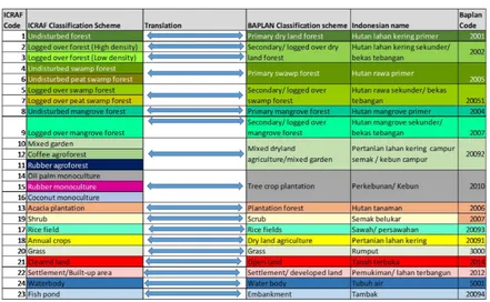
Figure 10: Conversion key between the ICRAF classification scheme and the BAPLAN classification scheme.

4.2.3.Land cover

(32)

[image:32.595.86.500.118.393.2]

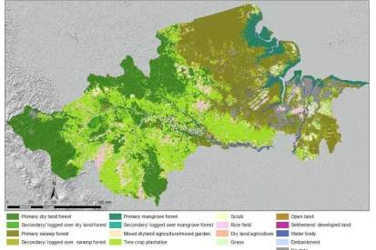
Figure 11: Land cover classification 1990.

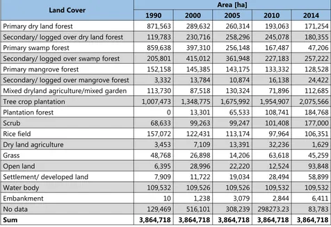
[image:32.595.92.493.434.721.2]

(33)

[image:33.595.52.528.137.464.2]

Table 8: Spatial extent of the different land cover categories in the five points in time.

Land Cover Area [ha]

1990 2000 2005 2010 2014

Primary dry land forest 871,563 289,632 260,314 193,063 171,254

Secondary/ logged over dry land forest 119,783 230,716 258,296 245,078 180,355

Primary swamp forest 859,638 397,310 256,148 167,487 47,206

Secondary/ logged over swamp forest 205,801 415,012 361,948 227,183 257,222

Primary mangrove forest 152,158 145,385 143,175 133,332 128,528

Secondary/ logged over mangrove forest 3,332 13,784 10,874 16,138 24,422 Mixed dryland agriculture/mixed garden 113,730 87,518 130,324 71,896 112,685 Tree crop plantation 1,007,473 1,348,775 1,675,992 1,954,907 2,075,566

Plantation forest 0 13,301 65,533 108,741 184,768

Scrub 68,633 99,263 99,247 101,408 177,000

Rice field 157,072 122,431 113,174 97,964 106,351

Dry land agriculture 3,453 7,109 13,391 32,236 1,629

Grass 48,768 26,898 14,206 63,618 45,259

Open land 6,395 28,996 22,220 12,524 93,848

Settlement/ developed land 7,909 11,722 19,034 28,494 58,899

Water body 109,532 109,526 109,526 109,532 109,532

Embankment 10 1,238 3,079 2,844 6,411

No data 129,469 516,101 308,239 298273.23 83,783

Sum 3,864,718 3,864,718 3,864,718 3,864,718 3,864,718

(34)

[image:34.595.55.530.132.476.2]

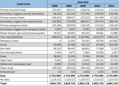
Table 9: Spatial extent of the different land cover categories after applying the common no data mask.

Land Cover Area [ha]

1990 2000 2005 2010 2014

Primary dry land forest 535,947 249,237 228,878 176,525 171,254

Secondary/ logged over dry land forest 86,219 211,542 173,755 178,190 136,500

Primary swamp forest 626,024 308,027 225,233 167,409 47,206

Secondary/ logged over swamp forest 156,004 279,509 280,437 187,474 189,734

Primary mangrove forest 145,296 140,039 139,139 133,332 128,528

Secondary/ logged over mangrove forest 2,597 6,654 6,781 11,420 13,579 Mixed dryland agriculture/mixed garden 54,025 66,681 86,243 46,081 75,986 Tree crop plantation 848,023 1,162,293 1,267,981 1,432,675 1,461,231

Plantation forest 0 13,301 34,243 56,704 107,682

Scrub 39,038 63,508 66,113 65,004 103,395

Rice field 99,119 90,402 86,901 77,084 72,310

Grass 38,081 16,209 9,296 50,598 30,296

Open land 4,645 19,353 13,664 10,121 57,574

Water body 109,526 109,526 109,526 109,526 109,526

Embankment 10 529 1,030 1,392 3,619

Sum 2,753,996 2,753,996 2,753,996 2,753,996 2,753,996

No data 1,110,722 1,110,722 1,110,722 1,110,722 1,110,722

Total 3,864,718 3,864,718 3,864,718 3,864,718 3,864,718

The most dominant land cover type in the study area was and is Tree crop plantation, occupying 848,023 ha in 1990 and expanding to 1,461,231 ha by 2014. The most abundant forest type in 1990 was Primary dryland forest with 535,947 ha, however this class lost about 68 % of its spatial extent until 2014 ending at 171,254 ha. Secondary dryland forest increased from 86,219 ha in 1990 to 211,542 ha in 2000, before decreasing until 2014. Primary peat swamp forest lost even more of its spatial extent, covering 626,024 ha in 1990, but only 47,206 ha in 2014. Large shares of these changes were due to forest degradation related to logging which is reflected by the increase of spatial extent of the Secondary/ logged over peat swamp forest. Most non forest classes experienced an increase in spatial extent, especially the plantation forest class, the mixed dryland agriculture class as well as the Settlement/ developed land class. A decrease in spatial extent was observed for the Rice field class.

4.2.4.Land cover change

(35)

[image:35.595.70.520.120.377.2]

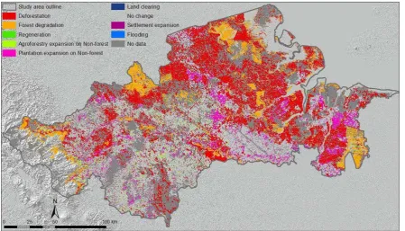
Figure 13: Land cover change 1990 – 2014.

Table 10: Land cover change in the five observation periods.

Land Cover

Area change (ha) 1990

-2000

2000 -2005

2005 -2010

2010 -2014

1990 -2014 Primary dry land forest -286,710 -20,358 -52,353 -5,271 -364,692 Secondary/ logged over dry land forest 125,322 -37,787 4,435 -41,689 50,281 Primary swamp forest -317,997 -82,794 -57,824 -120,203 -578,818 Secondary/ logged over swamp forest 123,504 928 -92,963 2,260 33,730

Primary mangrove forest -5,257 -900 -5,808 -4,804 -16,768

Secondary/ logged over mangrove forest 4,057 127 4,639 2,158 10,981 Mixed dryland agriculture/mixed garden 12,656 19,561 -40,161 29,904 21,960 Tree crop plantation 314,269 105,688 164,694 28,557 613,208

Plantation forest 13,301 20,942 22,460 50,978 107,682

Scrub 24,470 2,605 -1,109 38,391 64,357

Rice field -8,717 -3,501 -9,817 -4,773 -26,808

Dry land agriculture 3,634 1,787 18,062 -24,739 -1,256

Grass -21,872 -6,913 41,302 -20,302 -7,785

Open land 14,707 -5,689 -3,543 47,453 52,928

Water body 0 0 0 0 0

Embankment 519 500 363 2,227 3,608

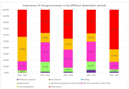
[image:35.595.91.510.439.763.2]

(36)

[image:36.595.68.523.304.659.2]

Table 11 and Figure 14 present a summary of the spatial extent of the different land cover change processes and the importance of those across the five observation periods. The importance of those changed intensively across time: While in the first period 1990 – 2000, deforestation and forest degradation were almost equal in importance (accounting for 43% and 39% of all observed changes), degradation declined to between 13 and 18% in the following periods. The reason is that apart from areas with a strict protection status (such as the National parks), the majority of primary forest have already experienced degradation in the earliest observation period. At the same time, Plantation expansion on Non-forest increased significantly from 14% (1990 – 2000) to approximately 29 – 31% in the following periods. In the overall observation period 1990 – 2014, deforestation accounted for 63% of all observed changes, forest degradation for 20%, Plantation expansion on Non-forest for 12% and Agroforestry expansion on Non-forest for 3.5%.

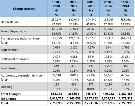
Table 11: Spatial extent of the gross land cover changes in the five observation periods.

Change process 1990 -2000 2000 -2005 2005 -2010 2010 -2014 1990 -2014

Ha Ha Ha Ha Ha

% % % % %

Deforestation 359,174 142,904 204,449 168,093 868,082

42.85% 36.74% 45.82% 37.38% 62.79%

Forest Degradation 326,720 57,921 78,060 59,842 275,702

38.98% 14.89% 17.50% 13.31% 19.94%

Plantation expansion on Non-forest

119,650 121,109 127,230 142,116 164,273

14.27% 31.14% 28.52% 31.60% 11.88%

Regeneration 2,094 2,120 4,576 544 2,796

0.25% 0.55% 1.03% 0.12% 0.20%

Settlement expansion 2,524 4,951 5,354 17,894 21,851

0.30% 1.27% 1.20% 3.98% 1.58%

Land clearing 449 419 135 1,277 340

0.05% 0.11% 0.03% 0.28% 0.02%

Agroforestry expansion on Non-forest

27,510 59,052 25,992 57,667 47,596

3.28% 15.18% 5.83% 12.82% 3.44%

Flooding 155 462 377 2,289 1,844

0.02% 0.12% 0.08% 0.51% 0.13%

(37)

[image:37.595.69.518.135.446.2]

Figure 14: Importance of change processes in the different observation periods.

4.2.5.Deforestation rate

Table 12 shows the net forest losses in the five observation periods. Between 1990 and 2000, 357,080 ha of forest have been lost which amounts to 23% of the forest cover at the start of the observation period. In the following periods, another 140,784 ha (12%), 199,873 ha (19%) and 167,549 ha (20%) have been lost. In the overall observation period 1990 – 2014, net forest loss amounted to 865,286 ha or 56% of the forest cover of 1990.

Table 12: Net forest loss in the five observation periods.

Net forest loss 1990 - 2000 2000 - 2005 2005 - 2010 2010 - 2014 1990 - 2014

ha -357,080 -140,784 -199,873 -167,549 -865,286

% -23.01% -11.78% -18.96% -19.61% -55.75%

(38)

[image:38.595.79.506.182.436.2]

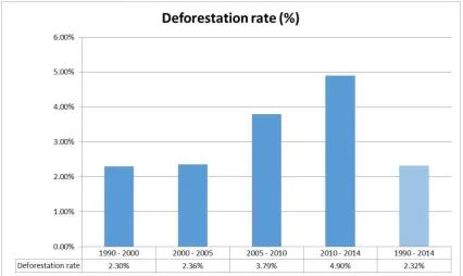
constant level (with a peak between 2005 and 2010), the spatial extent of forest cover diminished significantly. Therefore, the relative rates increase over time. In the overall observation period 1990 – 2014 the annual deforestation rate averaged at 2.3%.

Figure 15: Annual deforestation rate in the five observation periods.

(39)

Figure 16: Drivers of deforestation.

4.2.6.Carbon stock

To derive the carbon stock maps, the local aboveground biomass values derived in Work Package 3 (WP 3) were attributed to the different land cover classes. Carbon stock is reported in tons of carbon (t C). To calculate the carbon content of a certain stratum, the aboveground biomass value is simply divided by 2 (i.e. a carbon content of 0.5 is assumed). By multiplying the extent of the land cover by the carbon content per hectare per land cover class the total carbon stock of the respective land cover class is calculated (stratify & multiply approach).

Figure 17 and Figure 18 exemplary show the carbon stock maps for the years 1990 and 2014. The carbon stock of the land cover classes for the years 1990, 2000, 2005, 2010 and 2014 is shown in Table 13.

(40)

Figure 17: Carbon stock map 1990.

(41)

Table 13: Carbon stored in the different land cover classes at the five points in time.

Land Cover Carbon stock (t C)

1990 2000 2005 2010 2014

Primary dry land forest 146,045,443 67,917,009 62,369,356 48,103,114 46,666,832 Secondary/ logged over

dry land forest 11,036,091 27,077,322 22,240,581 22,808,287 17,472,038 Primary swamp forest 70,740,679 34,807,018 25,451,289 18,917,166 5,334,226 Secondary/ logged over

swamp forest 5,772,165 10,341,828 10,376,160 6,936,543 7,020,166

Primary mangrove forest 14,384,304 13,863,889 13,774,807 13,199,862 12,724,300 Secondary/ logged over

mangrove forest 57,139 146,393 149,191 251,250 298,729

Mixed dryland

agriculture/mixed garden 2,836,328 3,500,771 4,527,736 2,419,276 3,989,247 Tree crop plantation 13,568,373 18,596,684 20,287,692 22,922,794 23,379,703

Plantation forest 0 266,013 684,860 1,134,070 2,153,637

Scrub 487,970 793,847 826,416 812,553 1,292,438

Rice field 495,594 452,011 434,506 385,418 361,552

Grass 118,051 50,248 28,818 156,854 93,917

Open land 0 0 0 0 0

Settlement/ developed

land 0 0 0 0 0

Embankment 0 0 0 0 0

Sum 265,580,004 177,907,228 161,273,311 138,449,043 120,805,181

4.2.7.Carbon stock change

(42)

Table 14: Carbon stock change in the five observation periods.

Land Cover Carbon stock change (t C)

1990 - 2000 2000 - 2005 2005 - 2010 2010 - 2014 1990 - 2014 Primary dryland forest -78,128,434 -5,547,653 -14,266,242 -1,436,282 -99,378,611 Secondary/ logged over dryland

forest 16,041,231 -4,836,741 567,706 -5,336,248 6,435,948

Primary swamp forest -35,933,661 -9,355,729 -6,534,123 -13,582,940 -65,406,453 Secondary/ logged over swamp

forest 4,569,662 34,332 -3,439,617 83,623 1,248,001

Primary mangrove forest -520,415 -89,082 -574,944 -475,562 -1,660,004 Secondary/ logged over

mangrove forest 89,254 2,798 102,059 47,478 241,590

Mixed dryland agriculture/mixed

garden 664,444 1,026,965 -2,108,460 1,569,971 1,152,919

Tree crop plantation 5,028,312 1,691,008 2,635,102 456,909 9,811,331

Plantation forest 266,013 418,847 449,210 1,019,567 2,153,637

Scrub 305,877 32,569 -13,863 479,886 804,468

Rice field -43,583 -17,505 -49,087 -23,866 -134,042

Dryland agriculture 56,327 27,705 279,957 -383,460 -19,471

Grass -67,803 -21,430 128,036 -62,937 -24,134

Open land 0 0 0 0 0

Settlement/ developed land 0 0 0 0 0

Sum -87,672,776 -16,633,917 -22,824,268 -17,643,863 -144,774,823

(43)

[image:43.595.55.535.134.496.2]

Table 15: Annual carbon stock change in the five observation periods.

Land Cover Annual Carbon Emissions (t C yr-1)

1990 - 2000 2000 - 2005 2005 - 2010 2010 - 2014 1990 - 2014 Primary dry land forest -7,812,843 -2,219,061 -2,853,248 -359,071 -4,140,775 Secondary/ logged over dry land

forest 1,604,123 -1,934,696 113,541 -1,334,062 268,164

Primary swamp forest -3,593,366 -3,742,292 -1,306,825 -3,395,735 -2,725,269 Secondary/ logged over swamp

forest 456,966 13,733 -687,923 20,906 52,000

Primary mangrove forest -52,042 -35,633 -114,989 -118,891 -69,167

Secondary/ logged over

mangrove forest 8,925 1,119 20,412 11,870 10,066

Mixed dryland agriculture/mixed

garden 66,444 410,786 -421,692 392,493 48,038

Tree crop plantation 502,831 676,403 527,020 114,227 408,805

Plantation forest 26,601 167,539 89,842 254,892 89,735

Scrub 30,588 13,027 -2,773 119,971 33,520

Rice field -4,358 -7,002 -9,817 -5,967 -5,585

Dry land agriculture 5,633 11,082 55,991 -95,865 -811

Grass -6,780 -8,572 25,607 -15,734 -1,006

Open land 0 0 0 0 0

Settlement/ developed land 0 0 0 0 0

Sum -8,767,278 -6,653,567 -4,564,854 -4,410,966 -6,032,284

Figure 19 shows the analysis of the drivers of carbon emissions, as derived from the carbon change matrices of the emission assessment. The driver analysis is based on the class into which the land cover was converted in the respective time period, and it shows the emissions (or removals) resulting from the conversion, as well as the source of the emissions (i.e. which class was converted and how large the emissions from this class are.

(44)

[image:44.595.82.516.104.343.2]

Figure 19: Drivers of carbon emissions.

4.2.8.Carbon emission baseline

(45)

[image:45.595.70.517.100.370.2]

(46)

[image:46.595.80.507.194.574.2]

4.3. Work Package 2: Forest benchmark mapping and monitoring

Figure 21 shows the flowchart of the activities carried out in Work Package 1 (WP 1): Historic land cover change and carbon emission baseline.

Figure 21: Flow chart of the activities carried out in Work Package 2 (WP 2): Forest benchmark mapping and monitoring.

4.3.1.Dataset

Because it was not possible to cover the whole project area by SPOT images, it was necessary to acquire additional data with similar spectral and spatial characteristics. On this account also RapidEye data was used for generating the benchmark maps.

(47)

project areas with high resolution images. So it was decided to use Landsat 8 data to fill these missing parts. This way allows a founded analysis of land cover change also in areas without RapidEye data.

4.3.2.Preprocessing

The first step of the preprocessing was the geometric correction of the used SPOT-6 and RapidEye images. A geometric correction including orthorectification of the images was carried out based reference ground control points derived from the aerial photos collected during the LiDAR survey in October 2014 (which was referenced to a network of benchmarks of the Indonesian Geodetic Agency BIG) and Landsat satellite imagery (which was used in the historic land cover assessment by ICRAF). In order to apply terrain rectification, the digital elevation model (DEM) from the Shuttle Radar Topography Mission (SRTM) with a global resolution of 30 m was used. Based on the RPCs of the imagery, the GCPs and the DEM, a sensor specific model for SPOT-6 and RapidEye was used for geometric correction in the software ERDAS Imagine 2014.

The second step of the pre-processing was the removal of atmospheric distortions (scattering, illumination effects, adjacency effects), ind