CASE FAIR - 22 sd 25.rar

Prepared by:

Fernando & Yvonn

Quijano

22

Chapter

The Government

C

and Fiscal Policy

Government in the Economy

Government Purchases (G), Net Ta xes (T), and Disposable income (Y

d)

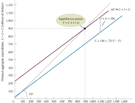
Equilibrium Output: Y = C + I + G

Fiscal Policy at Work: Multiplier Effects

The Government Spending Multiplier The Ta x Multiplier

The Balanced-Budget Multiplier

The Federal Budget

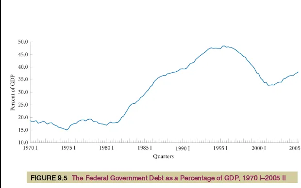
The Budget

The Surplus or Deficit The Debt

The Economy’s Influence on the Government Budget

C

THE GOVERNMENT AND FISCAL POLICY

fiscal policy

The government’s spending

and taxing policies.

monetary policy

The behavior of the

Federal Reserve concerning the nation’s

C

discretionary fiscal policy

Changes in

taxes or spending that are the result of

deliberate changes in government

C

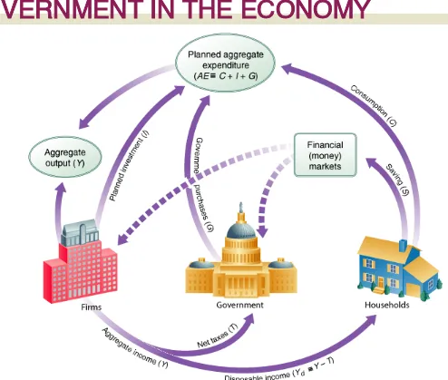
GOVERNMENT IN THE ECONOMY

GOVERNMENT PURCHASES (

G

), NET TAXES (

T

),

AND DISPOSABLE INCOME (

Y

_D

)

net taxes (

T

)

Ta xes paid by firms and

households to the government minus

transfer payments made to households

C

GOVERNMENT IN THE ECONOMY

disposable, or after-tax, income (

Y

_d

)

To tal income minus net taxes:

Y

−

T

.

disposable income

≡

total income

−

net taxes

C

When government enters the picture, the aggregate

income identity gets cut into three pieces:

C

GOVERNMENT IN THE ECONOMY

budget deficit

The difference between

what a government spends and what it

collects in taxes in a given period:

G

−

T

.

C

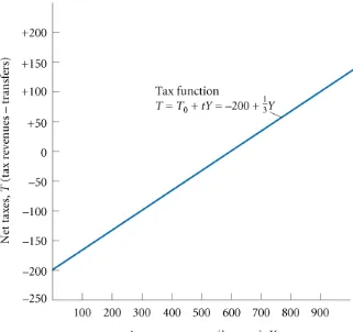
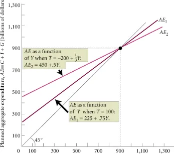
Adding Ta xes to the Consumption Function

To modify our aggregate consumption function to

incorporate disposable income instead of

before-tax income, instead of

C

=

a

+

bY

, we write

C

=

a

+

bY

_d

or

C

=

a

+

b

(

Y

−

T

)

Our consumption function now has consumption

depending on disposable income instead of

C

GOVERNMENT IN THE ECONOMY

Investment

C

(All Figures in Billions of Dollars)

(1) (2) (3) (4) (5) (6) (7) (8) (9) (10)

300 100 200 250

 50 100 100 450  150 Output



500 100 400 400 0 100 100 600 _

100 Output



700 100 600 550 50 100 100 750

 50 Output



900 100 800 700 100 100 100 900 0 Equilibrium 1,100 100 1,000 850 150 100 100 1,050 + 50

Output



1,300 100 1,200 1,000 200 100 100 1,200 + 100

Output



1,500 100 1,400 1,150 250 100 100 1,350 + 150

C

GOVERNMENT IN THE ECONOMY

C

The Leakages/Injections Approach to Equilibrium

leakages/injections approach to equilibrium:

S

+

T

=

I

+

G

Ta xes (

T

) are a leakage from the flow of income. Saving

(

S

) is also a leakage.

In equilibrium, aggregate output (income) (

Y

) equals

C

FISCAL POLICY AT WORK:

MULTIPLIER EFFECTS

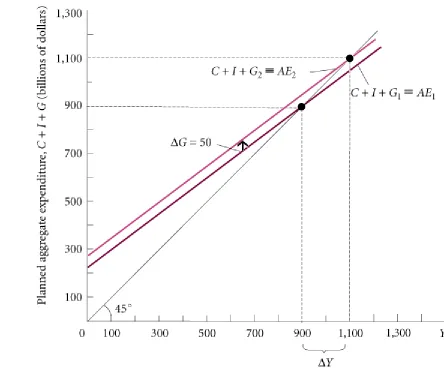
THE GOVERNMENT SPENDING MULTIPLIER

TABLE 9.2

Finding Equilibrium After a $50 Billion Government Spending Increase (All

Figures in Billions of Dollars; G Has Increased from 100 in Ta ble 9.1 to

150 Here)

300 100 200 250

 50 100 150 500  200 Output



500 100 400 400 0 100 150 650

 150 Output



700 100 600 550 50 100 150 800

 100 _Output



900 100 800 700 100 100 150 950

 50 Output



1,100 100 1,000 850 150 100 150 1,100 0 Equilibrium 1,300 100 1,200 1,000 200 100 150 1,250 + 50

C

government spending multiplier

The

ratio of the change in the equilibrium

level of output to a change in

C

FISCAL POLICY AT WORK:

MULTIPLIER EFFECTS

C

THE TAX MULTIPLIER

tax multiplier

The ratio of change in

the equilibrium level of output to a

change in taxes.

C

FISCAL POLICY AT WORK:

C

THE BALANCED-BUDGET MULTIPLIER

balanced-budget multiplier

The ratio of

change in the equilibrium level of

output to a change in government

spending where the change in

government spending is balanced by a

change in taxes so as not to create any

deficit. The balanced-budget multiplier

is equal to 1: The change in

Y

resulting from the change in

G

and the

equal change in

T

is exactly the same

size as the initial change in

G

or

T

C

FISCAL POLICY AT WORK:

MULTIPLIER EFFECTS

C

TABLE 9.3

Finding Equilibrium After a $200-Billion Balanced-Budget Increase in G

and T (All Figures in Billions of Dollars; Both G and T Have Increased

from 100 in Ta ble 9.1 to 300 Here)

500 300 200 250 100 300 650

 150 Output



700 300 400 400 100 300 800

 100 Output



900 300 600 550 100 300 950

 50 Output



1,100 300 800 700 100 300 1,100 0 Equilibrium 1,300 300 1,000 850 100 300 1,250 + 50

Output



1,500 300 1,200 1,000 100 300 1,400 + 100

C

FISCAL POLICY AT WORK:

MULTIPLIER EFFECTS

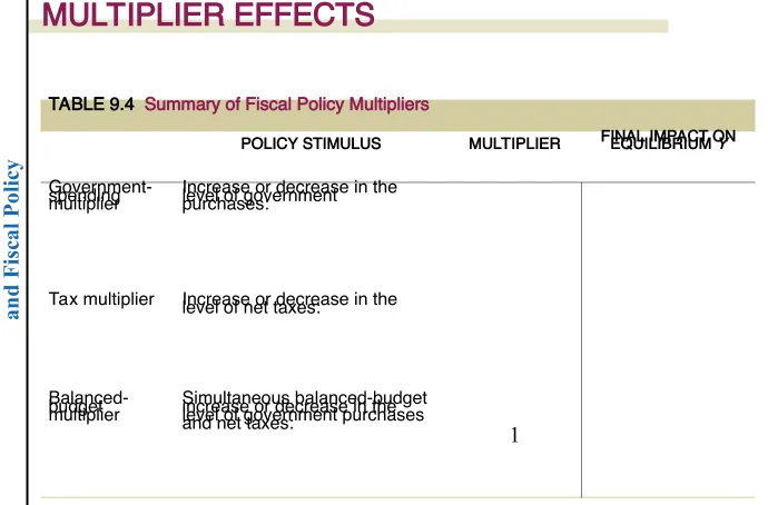
TABLE 9.4

Summary of Fiscal Policy Multipliers

POLICY STIMULUS

MULTIPLIER

FINAL IMPACT ON

EQUILIBRIUM Y

Government-spending

multiplier

Increase or decrease in the

level of government

purchases:

Ta x multiplier

Increase or decrease in the

level of net taxes:

Balanced-budget

multiplier

Simultaneous balanced-budget

increase or decrease in the

level of government purchases

and net taxes:

C

C

THE FEDERAL BUDGET

THE BUDGET

TABLE 9.5

Federal Government Receipts and Expenditures, 2004 (Billions of Dollars)

AMOUNT

PERCENTAGE

OF TOTAL

Receipts

Personal income taxes 801.8 40.6

Excise taxes and custom duties 94.0 4.8

Corporate income taxes 217.4 11.0

Ta xes from the rest of the world 9.2 0.5

Contributions for social insurance 802.5 40.6

Interest receipts and rents and royalties 21.9 1.1

Current transfer receipts from business and persons 28.6 1.4

Current surplus of government enterprises − 0.5 0.0

To tal 1,974.8 100.0

Current Expenditures

Consumption expenditures 725.7 30.5

Transfer payments to persons 1,014.0 42.6

Transfer payments to the rest of the world 28.9 1.2

Grants-in-aid to state and local governments 348.3 14.6

Interest payments 221.5 9.3

Subsidies 43.0 1.8

To tal 2,381.3 100.0

Net federal government saving—surplus (+) or deficit (

−

)

C

THE SURPLUS OR DEFICIT

federal surplus (+) or deficit (

−

)

Federal

government receipts minus expenditures.

C

THE FEDERAL BUDGET

THE DEBT

federal debt

The total amount owed

by the federal government.

privately held federal debt

The

privately held (nongovernment-

C

C

THE ECONOMY’S INFLUENCE

ON THE GOVERNMENT BUDGET

TAX REVENUES DEPEND ON THE STATE OF THE

ECONOMY

C

SOME GOVERNMENT EXPENDITURES DEPEND

ON THE STATE OF THE ECONOMY

Transfer payments tend to go down

automatically during an expansion.

Inflation often picks up when the economy is

expanding. This can lead the government to

spend more than it had planned to spend.

C

THE ECONOMY’S INFLUENCE

ON THE GOVERNMENT BUDGET

AUTOMATIC STABILIZERS

automatic stabilizers

Revenue and

expenditure items in the federal

budget that automatically change

with the state of the economy in

C

fiscal drag

The negative effect on

the economy that occurs when

average tax rates increase because

taxpayers have moved into higher

income brackets during an

C

THE ECONOMY’S INFLUENCE

ON THE GOVERNMENT BUDGET

FULL-EMPLOYMENT BUDGET

full-employment budget

What the

federal budget would be if the

economy were producing at a

full-employment level of output.

structural deficit

The deficit that

remains at full employment.

cyclical deficit

The deficit that

occurs because of a downturn in the

C

discretionary fiscal policy

disposable, or after-tax,

income (Y

_d

)

federal budget

federal debt

federal surplus (+) or

deficit (

−

)

fiscal drag

fiscal policy

full-employment budget

government spending

net taxes (T)

privately held federal debt

structural deficit

tax multiplier

1.

Disposable income Yd

≡

Y

−

T

2.

AE

≡

C + I + G

3.

Government budget deficit

≡

G

−

T

4.

Equilibrium in an economy with

government: Y = C + I + G

5.

Leakages/injections approach to

equilibrium in an economy with

government: S + T = I + G

6.

Government spending multiplier

≡

7.

Ta x multiplier

≡

C

DERIVING THE FISCAL POLICY MULTIPLIERS

Appendix A

THE GOVERNMENT SPENDING AND TAX

C

THE BALANCED-BUDGET MULTIPLIER

The balanced-budget multiplier is found by combining

the effects of government spending and taxes:

increase in spending:

- decrease in

spending:

= net increase in spending

In a balanced-budget increase,

Δ

G

=

Δ

T

, so we can

substitute:

net initial increase in spending:

C

THE CASE IN WHICH TAX REVENUES DEPEND ON

C

C

THE GOVERNMENT SPENDING AND TAX