Effects of spatial variability of soil properties on slope stability
Sung Eun Cho
⁎
Dam Engineering Research Center, Korea Institute of Water and Environment, Korea Water Resources Corporation, 462-1, Jeonmin-Dong, Yusung-Gu, Daejon 305-730, South Korea
Received 22 November 2006; received in revised form 7 March 2007; accepted 20 March 2007 Available online 5 April 2007
Abstract
Slope stability analysis is a geotechnical engineering problem characterized by many sources of uncertainty. Some of the uncertainties are related to the variability of soil properties involved in the analysis. In this paper, a numerical procedure for a probabilistic slope stability analysis based on a Monte Carlo simulation that considers the spatial variability of the soil properties is presented. The approach adopts the first-order reliability method to determine the critical failure surface and to conduct preliminary sensitivity analyses. The performance function was formulated by Spencer's limit equilibrium method to calculate the reliability index defined by Hasofer and Lind. As examples, probabilistic stability assessments were performed to study the effects of uncertainty due to the variability of soil properties on slope stability in layered slopes. The examples provide insight into the application of uncertainty treatment to the slope stability and show the importance of the spatial variability of soil properties with regard to the outcome of a probabilistic assessment.
© 2007 Elsevier B.V. All rights reserved.
Keywords:Slope stability; Spatial variability; Monte Carlo simulation; Reliability index; Probability
1. Introduction
Soil properties vary spatially even within homoge-neous layers as a result of depositional and post-depositional processes that cause variation in properties (Lacasse and Nadim, 1996). Nevertheless, most geo-technical analyses adopt a deterministic approach based on single soil parameters applied to each distinct layer. The conventional tools for dealing with ground hetero-geneity in the field of geotechnical engineering have been applied under the use of safety factors and by implementing local experience and engineering judg-ment (Elkateb et al., 2002). However, it has been recognized that the factor of safety is not a consistent
measure of risk since slopes with the same safety factor value may exhibit different risk levels depending on the variability of the soil properties (Li and Lumb, 1987). Accordingly, numerous studies have been undertaken in recent years to develop a probabilistic slope stability analysis that deals with the uncertainties of soil properties in a systematic manner (Alonso, 1976; Vanmarcke, 1977b; Li and Lumb, 1987; Christian et al., 1994; Griffiths and Fenton, 2004). Detailed reviews of these studies can be
found inMostyn and Li (1993),El-Ramly et al. (2002), and
Baecher and Christian (2003).
Unfortunately, probabilistic slope stability analysis methods do not consider all of the components of slope design where judgment needs to be utilized and they also do not suggest the level of reliability that should be targeted (D'Andrea, 2001). However, working within a probabilistic framework does offer the advantage that www.elsevier.com/locate/enggeo
⁎ Tel.: +82 42 870 7632; fax: +82 42 870 7639.
E-mail address:[email protected].
the reliability of the system can be considered in a logical manner. Thus, probabilistic models can facilitate the development of new perspectives concerning risk and reliability that are outside the scope of conventional deterministic models.
In this study, a procedure for a probabilistic slope stability analysis is presented. The procedure is based on a Monte Carlo simulation to compute a probability dis-tribution of the resulting safety factors. The analysis considers the spatial variability of soil properties based on local averaging to discretize continuous random fields.
An essential component of the procedure is the de-termination of the critical failure surface. The approach presented herein adopts the first-order reliability method (FORM) to determine the critical probabilistic surface and to conduct preliminary sensitivity analyses. The latter are used to identify model input parameters that make important contributions to the stability. The method is based on the stability model presented by Spencer (1967)for the formulation of the performance function to calculate the reliability index, defined by Hasofer and Lind (1974). The index gives an invariant risk measure, and hence all equivalent formats of the performance function yield the same reliability index (Li and Lumb, 1987).Low and Tang (1997)andLow et al. (1998) have used a spreadsheet reliability evaluation method based on the intuitive ellipsoidal perspective in the original space of the random variables to calculate
the Hasofer–Lind reliability index.
This study focuses primarily on inherent soil vari-ability, where probabilistic analyses can be employed to assess the effect of this type of variability on slope stability. The importance of the spatial correlation struc-ture of soil properties is highlighted and its effect on the stability of slope is studied.
2. Slope stability analysis
2.1. Limit equilibrium method
Slope stability problems are commonly analyzed using limit equilibrium methods of slices. The failing soil mass is divided into a number of vertical slices to calculate the factor of safety, defined as the ratio of the resisting shear strength to the mobilized shear stress to maintain static equilibrium. The static equilibrium of the slices and the mass as a whole are used to solve the problem. However, all methods of slices are statically indeterminate and, as a result, require assumptions in
order to solve the problem.Spencer (1967)developed a
slope stability analysis technique based on the method of slices that satisfies both force and moment
equilib-rium for the mass as a whole. The approach presented herein adopts Spencer's method and is applicable to a failure surface of an arbitrary shape.
2.2. Search for the critical deterministic surface
Limit equilibrium methods require that the critical failure surface be determined as part of the analysis. The problem of locating the critical surface can be for-mulated as a constrained optimization problem, and the noncircular slip surface is generated by a series of straight lines of which the vertices are considered as shape variables.
min
surfaceFðxÞ subject to some kinematical constraints
ð1Þ
where F(x) is the objective function and x is a shape
variable vector defining the location of the slip surface. In the problem of finding the critical deterministic surface, the objective function is defined as the factor of safety associated with variables of the coordinates that describe the geometry of a slip surface and mean-values of soil parameters. In previous works, many optimization techniques have been applied to search for the critical surface. In recent years, some global optimization methods also have been applied to the slope stability problem (Bolton et al., 2003; Cheng, 2003; Zolfaghari et al., 2005). In this study, to solve the constrained optimization problem, the feasible direction method, moving from a feasible point to an improved feasible point along the feasible direction, is used.
An improved search strategy, proposed by Li and
White (1987) and Greco (1996), is used for a noncircular critical surface. The approach starts with a search method for a circular critical surface, since poor results frequently occur when a relatively large number of variables are used in the initial guess. During the search process, new vertices are successively introduced at midpoints of straight lines joining adjacent vertices, and the points defining a trial slip surface are moved in two-dimensional space subject to some kinematical constraints to make the slip surface smooth. A new search starts with the critical slip surface in the previous
search step as the trial slip surface for the next.Kim and
Lee (1997)have presented a detailed description of this procedure.
3. Probabilistic slope stability analysis
the determination of the exact system reliability of the slope stability problem is not possible. Therefore, the probability of the most critical slip surface is commonly used as the estimate of the system failure probability. This approach assumes the probability of failure along different slip surfaces is highly correlated (Mostyn and Li, 1993; Chowdhury and Xu, 1995).
A common approach to a probabilistic analysis is to locate the critical deterministic surface and then calculate the probability of failure corresponding to this surface. However, the surface of the minimum factor of safety may not be the surface of the maximum probability of failure (Hassan and Wolff, 1999).
As an alternative, the critical probabilistic surface that is associated with the highest probability of failure or the lowest reliability could be considered (Li and Lumb, 1987; Chowdhury and Xu, 1995; Liang et al., 1999; Bhattacharya et al., 2003). The search for the critical probabilistic surface is not different in concept from that of the deterministic critical surface. The prob-lem of locating the critical probabilistic surface can be
performed by minimizing a reliability indexβassociated
with a set of geotechnical parameters including the statistical properties.
There have been numerous discussions on the prob-lem of locating the critical probabilistic surface asso-ciated with the maximum probability of failure (Hassan and Wolff, 1999; Li and Cheung, 2001; Bhattacharya et al., 2003).
3.1. Performance function
The problem of the probabilistic analysis is
formu-lated by a vector,X= [X1,X2,X3,…,Xn], representing a set
of random variables. From the uncertain variables, a
performance functiong(X) is formulated to describe the
limit state in the space of X. In n-dimensional
hyper-space of the basic variables, g(X) = 0 is the boundary
between the region in which the target factor of safety is not exceeded and the region in which it is exceeded. The probability of failure of the slope is then given by the following integral:
Pf ¼P½gðXV0Þ ¼
Z
gðXÞV0
fXðXÞdX ð2Þ
where fX(X) represents the joint probability density
function and the integral is carried out over the failure domain.
For slope stability problems, direct evaluation of the n-fold integral is virtually impossible. The difficulty lies in that complete probabilistic information on the soil
properties is not available and the domain of integration is a complicated function. Therefore, approximate tech-niques have been developed to evaluate this integral.
The performance function for the slope stability is usually defined as
gðXÞ ¼Fs 1:0 ð3Þ
The method of stability analysis proposed by Spencer is used to describe the above performance function by
calculatingFsfor the failure surface.
3.2. First-order reliability method
The first-order reliability evaluation of Eq. (2) is
ac-complished by transforming the uncertain variables,X,
into uncorrelated standard normal variables,Y. The
pri-mary contribution to the probability integral in Eq. (2)
comes from the part of the failure region (G(Y)≤0, where
G(Y) is the performance function in the transformed
normal space) closest to the origin. The design point is
defined as the pointY⁎in the standard normal space that
is located on the performance function (G(Y) = 0) and
having maximum probability density attached to it. Therefore, the design point, which is the nearest point to
the origin in the failure region (G(Y)≤0), is an optimum
point at which to approximate the limit state surface. The probability approximated at the design point is:
P½gðXÞV0cUð bÞ ð4Þ
whereβ is the reliability index, defined by the distance
from the origin to the design point, andΦis the standard
normal cumulative density function.
In the first-order reliability method, a tangent hyper plane is fitted to the limit state surface at the design point. Therefore, the most important and demanding step in the method is finding the design point. The design point is the solution of the following nonlinear constrained optimization problem:
minjjYjj subject toGðYÞ ¼0 ð5Þ
Several algorithms have been proposed for the solu-tion of this problem (Hasofer and Lind, 1974; Rackwitz and Fiessler, 1978; Liu and Der Kiureghian, 1990).
As a by-product of the first-order reliability method, we can evaluate the measures of sensitivity of the reli-ability index with respect to the basic random variables. These sensitivity measures identify the random variables that have the greatest impact on the failure probability.
The unit vector,α, normal to the limit state surface at
measure that describes the sensitivity of the reliability index, with respect to variations in each of the standard variates.
~¼jY⁎b ð6Þ
For the first-order reliability analysis, FERUM
(Finite Element Reliability Using Matlab, http://www.
ce.berkeley.edu/FERUM) developed at the University
of California at Berkeley byHaukaas and Der Kiuregian
(2001)is used through direct coupling with the slope stability analysis routine written in FORTRAN.
3.3. Monte Carlo simulation
An alternative means to evaluate the multi-dimen-sional integral of Eq. (2) is the use of a Monte Carlo simulation. In a Monte Carlo simulation, discrete values of the component random variables are generated in a fashion consistent with their probability distribution, and the performance function is calculated for each generated set. The process is repeated many times to obtain an approximate, discrete probability density function of the performance function.
Several sampling techniques, also called variance reduction techniques, have been developed in order to improve the computational efficiency of the method by reducing the statistical error inherent in Monte Carlo methods and keeping the sample size to the minimum
possible. A detailed review can be found inBaecher and
Christian (2003). Among them Latin hypercube sam-pling may be viewed as a stratified samsam-pling scheme designed to ensure that the upper or lower ends of the distributions used in the analysis are well represented. Latin hypercube sampling is considered to be more efficient than simple random sampling, that is, it
re-quires fewer simulations to produce the same level of precision. Latin hypercube sampling is generally recommended over simple random sampling when the model is complex or when time is an issue.
In this study, the Latin Hypercube sampling tech-nique is used to generate random properties of soil. In
particular, the method proposed by Stein (1987) for
sampling dependent variables based on the rank of a target multivariate distribution with a local averaging method is implemented in Matlab.
4. Discretization of random fields
Soils are highly variable in their properties and rarely homogeneous by nature. One of the main sources of heterogeneity is inherent spatial soil variability, i.e., the variation of soil properties from one point to another in space due to different deposition conditions and dif-ferent loading histories (Elkateb et al., 2002). Spatial variations of soil properties can be effectively described by their correlation structure within the framework of random fields (Vanmarcke, 1983).
Most numerical solution algorithms require that all continuous parameter fields be discretized. When spatial uncertainty effects are directly included in the analysis, it is reasonable to use random fields for a more accurate representation of the variations. The spatial fluctuations of a parameter cannot be accounted for if the parameter is modeled by only a single random variable.
The midpoint method, the simplest method of dis-cretization, has been used to handle the spatial variation of soil properties (Auvinet and González, 2000; Low, 2003). In this method the field within one segment is described by a single random variable, which represents the field value at the centroid of the segment base.
Consequently, the discretized field is a step-wise con-stant with discontinuities at the segment boundaries.
The stability of a soil slope tends to be controlled by the averaged soil strength rather than the soil strength at a particular location along the slip surface, since soils generally exhibit plastic behavior (Li and Lumb, 1987). The variance of the strength spatially averaged over some domain is less than the variance of point mea-surements used for the midpoint method. As the extent of the domain over which the soil property is being averaged increases, the variance decreases (El-Ramly et al., 2002).
The effect of spatial averaging and spatial autocor-relation of soil properties on the stability of the slope has been noted in the literature (Vanmarcke, 1977a; Li and Lumb, 1987; El-Ramly et al., 2002). In the local aver-aging method, the field within each segment is described in terms of the spatial average of the field over the segment base. The discretized field is still constant over each segment with step-wise discontinuities at the segment boundaries, but a better fit can be expected due to the averaging process.
In this study, a local averaging method combined with numerical integration is adopted to discretize both isotropic and anisotropic random fields of soil properties in two-dimensional space.
4.1. Variance function
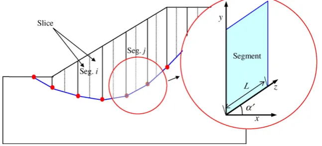
From a continuous two-parameter stationary
ran-dom fieldU(x,y) having a linear relationship between
parameters, as shown in Fig. 1, a family of moving
average processes is formed as follows (Knabe et al., 1998):
where L denotes the averaged length. The averaging
operation will not change the expected value U_ while
the variance of the moving average processσUL
2
where σU2 is the point variance of the random fieldU
andγ(L) is the variance function bounded by 0 and 1;
that is to say, the variance of the averaged soil property is in general less than the variance of the point property (Li and Lumb, 1987).
The variance function is related to the correlation function as follows (Vanmarcke, 1977a):
gðLÞ ¼Cor½L;L ¼
Vanmarcke (1977a) observed that γ(L) becomes
inversely proportional to L at large values of L, and
refers to the proportionality constant as the scale of
fluctuation,δ:
d¼ lim LYl½L
gðLÞ ð10Þ
This is a measure of the spatial extent within which soil
properties show a strong correlation. A large value ofδ
implies that the soil property is highly correlated over a Table 1
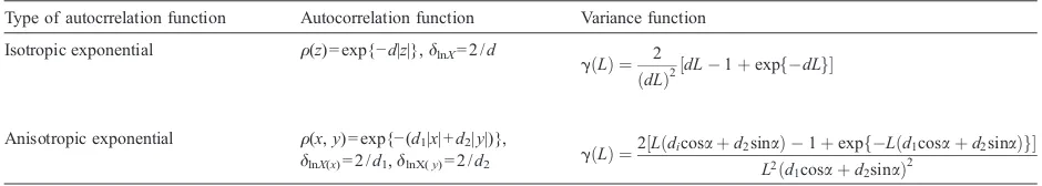
Exact spatial variance functions for two autocorrelation functions
Type of autocrrelation function Autocorrelation function Variance function
Isotropic exponential ρ(z) = exp{−d|z|},δlnX= 2 /d δlnX(x)is the horizontal scale of fluctuation, andδlnX(y)is the vertical scale of fluctuation.
large spatial extent, resulting in a smooth variation within the soil profile. On the other hand, a small value indicates that the fluctuation of the soil property is large (Li and Lumb, 1987). Variance functions for two commonly applied correlation functions in engineering (Table 1) are used in this study.
4.2. Correlation of local averages
In a probabilistic analysis, the spatial variability of soil properties is described using a correlation function. By averaging the random field over the arbitrarily
situated segmentsLi and Lj, as shown in Fig. 2, local
averages are defined. The correlation between these variables can be calculated by averaging the correlation between random variables at all points on both segments.
Since analytical results of Eq. (11) are difficult to obtain, integrations have to be performed numerically (Knabe et al., 1998; Rackwitz, 2000). In this study, the
numerical integration scheme presented byKnabe et al.
(1998)is used to calculate the correlation.
For two arbitrarily located segments with end points
of known coordinates (Fig. 2), the anglesα′andβ′of
straight lines inclined to the horizontal are as follows:
aV¼tan 1 ykðiÞ ypðiÞ
where xp,ypare the coordinates of the beginning of a
segment and xk, ykare the coordinates of the end of a
segment.
The distance z between two arbitrarily situated
points, one on segmentiand another on segmentj, is:
z¼
ffiffiffiffiffiffiffiffiffiffiffiffiffiffiffiffiffiffiffiffiffiffiffiffiffiffiffiffiffiffiffiffiffiffiffiffiffiffiffiffiffiffiffiffiffiffiffiffiffiffiffiffiffiffiffiffiffiffiffiffiffiffiffiffiffiffiffiffiffiffiffiffiffiffiffiffiffiffiffiffiffiffiffiffiffiffiffiffiffiffiffiffiffiffiffiffiffiffiffiffiffiffiffiffiffiffiffiffiffiffiffiffiffiffiffiffiffiffiffiffiffiffiffiffiffiffi
½tanbVðxðjÞ xpðjÞÞ tanaVðxðiÞ xpðiÞÞ þyp2þ ðxðjÞ xðiÞÞ2
q
ð13Þ
Eq. (11) then takes the following form:
Cor ULi;ULj
In this section, application of the presented procedure is illustrated through an analysis of example problems to Fig. 3. Example 1: Cross-section and searched critical slip surfaces.
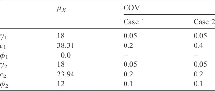
Table 2
Example 1: Statistical properties of soil parameters (based onHassan and Wolff, 1999)
evaluate the effect of spatial variability of soil param-eters on the probability of failure.
All variables are assumed to be characterized
statis-tically by a lognormal distribution defined by a meanμX
and a standard deviationσX. The lognormal distribution
ranges between zero and infinity, skewed to the low range, and hence is particularly suited for parameters that cannot take on negative values. Once the mean and standard deviation are expressed in terms of the
dimen-sionless coefficient of variation (COV), defined asVX=
σX/μX, then the mean and standard deviation of the
lognormal distribution are given by
rlnX ¼
All the random variables are regarded as independent as this assumption simplifies the computation and also gives conservative results (Li and Lumb, 1987) if cohesion and friction angle are negatively correlated.
The statistics of the underlying lognormal field, including local averaging, are given by (Griffiths and Fenton, 2004)
r2lnXA¼r2lnXgðLÞ ð17Þ
llnXA¼llnX ð18Þ
whereμlnXAis the locally averaged mean andσlnXAis
the locally averaged standard deviation of lnX.
In the current study, the scale of fluctuationδlnXis
considered for the spatial discretization of the lognormal random field. Although different values of the scale of fluctuation can be used for each random variable, they are assumed to be equal in this study. The locally
averaged meanμXAand standard deviationσXAover the
segment on the failure surface are given by
lXA¼expðllnXAþ0:5r
The discretization of a spatially distributed random field is performed by discretizing the slope into several segments and specifying a set of correlated random variables such that each random variable represents the random field over a particular segment.
5.1. Example 1: Application to a two-layered slope
In this example, a series of parametric studies are performed on a two-layered slope with a cross-section as
shown in Fig. 3. The basic soil parameters that are
related to the stability of slope, including unit weight, friction angle, and cohesion, are considered as random
variables.Table 2 summarizes the statistical properties
of soil parameters for two different coefficients of variation of cohesion in the upper layer.
The minimum factor of safety associated with the critical deterministic surface based on the mean values of soil properties is 1.592 and the surface passes through
the lower soil layer as presented inFig. 3. The critical
probabilistic surface, as determined by a search of FORM, passes through the upper layer where the vari-ation of shear strength is large, since the surface is associated with the maximum probability of failure. Searched probabilistic surfaces for the two cases show
almost the same locations.Table 3presents the results
obtained from FORM, i.e., the sensitivities, the reliabil-ity index, and the probabilreliabil-ity of failure. The sensitivities show the relative importance of the uncertainty in each random variable.
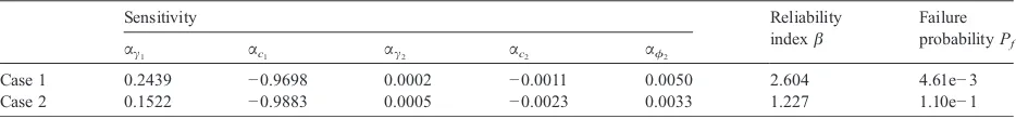
Table 4presents the results calculated from a Monte Carlo simulation for the previously located critical Table 3
Example 1: Results of FORM
Sensitivity Reliability
indexβ
Failure probabilityPf αγ1 αc1 αγ2 αc2 αϕ2
Case 1 0.2439 −0.9698 0.0002 −0.0011 0.0050 2.604 4.61e−3
Case 2 0.1522 −0.9883 0.0005 −0.0023 0.0033 1.227 1.10e−1
Table 4
Example 1: Results of Monte Carlo simulation assuming perfect spatial correlation
μFS 1.7364 1.7350 1.5954 1.5948
σFS 0.3582 0.7001 0.1917 0.3152
Pf 4.64e−3 1.10e−1 2.00e−5 3.17e−3
surfaces assuming a perfect spatial correlation. Al-though the mean factors of safety in the critical deter-ministic surface are lower, the probabilities of failure are
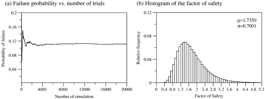
higher in the critical probabilistic surface.Figs. 4 and 5
show the results related to the critical probabilistic surface. Relatively good agreement with those obtained from FORM is noted.
Figs. 4(a) and 5(a) show the convergence of the simulations. As expected, considerably more trial runs are required for convergence in the case of a small probability of failure.
In the next step, the spatial variability of soil param-eters is considered in a Monte Carlo simulation for the critical probabilistic surface of case 2. The length of the critical probabilistic surface is 28.5 m and the surface is divided into several segments by grouping slices. The variance function of each segment is calculated by Eq. (9)
and the correlation coefficients between segments are estimated using Eq. (14). The Monte Carlo simulation is performed using a data set sampled based on the statistical information.
Fig. 6shows the probability distribution of the factor of safety with the variation of the scale of fluctuation for an isotropic random field. The figure indicates that the factor of safety is distributed in a wider range with
increased δlnX, since the spatial variation of soil
properties does not significantly affect the mean factor of safety, but has a very significant effect on the standard deviation of the factor of safety.
Fig. 7shows the probability distribution of the factor of safety with variation of the vertical scale of
fluctuation for fixed δlnX(x) (= 10 m), when the
anisotropic autocorrelation function is considered. The results also show a similar trend with the case of an Fig. 4. Example 1: Results of Monte Carlo simulation (Case 1).
isotropic random field. When the ratio ofδlnX(x)/δlnX(y) becomes 1.0, the curve is almost identical to that of the isotropic case.
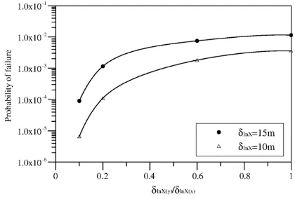
The effects of the scale of fluctuation on the
probability of failure are summarized in Figs. 8 and 9
for isotropic and anisotropic random fields, respectively. As indicated in the figure, the probability of failure decreases with a decrease in the scale of fluctuation, which would be expected, as the smaller scale of fluc-tuation leads to a smaller uncertainty in the average strength value across the failure surface. The weak cor-relation induces significant fluctuation of the sampled soil properties along the slip surface. Therefore, the probability of trial runs with a factor of safety of less
than 1.0 decreases since the fluctuations are averaged to a mean value along the whole failure surface. On the contrary, the probability of failure increases with in-creasing the scale of fluctuation. This is to be expected, since a higher scale of fluctuation value indicates that the random variables are more strongly correlated. Thus, the infinite value of the scale of fluctuation implies a perfectly correlated random field, or a single random variable, and gives the maximum value of the
prob-ability of failure.Fig. 9also shows that the assumption
of isotropic random field is conservative.
5.2. Example 2: Application to the Sugar Creek embankment fill slope
This example concerns the stability of the Sugar
Creek embankment fill slope reported in White et al.
(2005). Geotechnical investigation and characterization were performed on the site to determine the subsurface stratification and the shear strengths of the soils. A Fig. 6. Example 1: Variation of probability distribution of the factor of
safety withδlnX(isotropic random field).
Fig. 7. Example 1: Variation of probability distribution of the factor of safety withδlnX(x)/δlnX(y)(δlnX(x)= 10 m, anisotropic random field).
Fig. 8. Influence of scale of fluctuation on the probability of failure (isotropic random field).
typical slope section showing the soil profile and water
table is presented inFig. 10. The subsurface soils of the
site were roughly divided into the alluvium layer and the underlying shales. The shales were classified according to weathering grades in three layers of shales: highly weathered shale, moderately weathered shale, and slightly weathered shale. All the shales were classified as either low plasticity clay (CL) or high plasticity clay (CH) according to USCS.
The shear strength parameter values obtained from a BST (Borehole Shear Test), which gives the shear strength of in-situ, undisturbed soils, were used for the slope stability analysis. Uncertainty in pore water pres-sure was not considered in this analysis and the pie-zometric lines were treated as deterministic values, since
the sensitivity analysis results given by White et al.
(2005)indicated that, within the range of variation of the water level in the creek, the variation of the factor of safety for slope is insignificant. The statistical properties
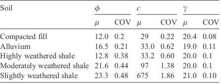
of the soil parameters are given inTable 5.
The factor of safety associated with the critical
deter-ministic surface is 1.615.Fig. 10 shows the searched
critical surfaces. They show somewhat different loca-tions, but pass through the relatively weak layer of the
highly weathered shale. Table 6 presents the FORM
results. The moderately weathered shale and slightly weathered shale appear to have essentially no effect on the slope stability, in spite of substantial variations in cohesion, since the strength of these layers is much higher than that of the overlying soils. This is supported
by the sensitivities presented inTable 6.
In the second step, the spatial variability of the soil parameters is considered in a Monte Carlo simulation for the critical probabilistic surface based on the spatial-ly averaged random variables.
According to the FORM results, the sensitivities of the unit weight are relatively small compared to those of the other variables; hence the unit weight is treated in a deterministic manner in this example, which decreases computational effort drastically.
As the scale of fluctuation is not known in this site, the sensitivity of the probability of failure to the scale of fluctuation is examined. When the probability of failure is too sensitive to the scale of fluctuation, additional efforts are needed to estimate the correlation structure on
dominant layer of stability. According toEl-Ramly et al.
(2003), horizontal scales of fluctuation that are relevant to slope stability are typically between 20 and 80 m Fig. 10. Example 2: Cross-section and searched critical slip surfaces for Sugar Creek embankment.
Table 5
Example 2: Statistical properties of soil parameters for Sugar Creek embankment (based onWhite et al., 2005)
Soil ϕ c γ
μ COV μ COV μ COV
Compacted fill 12.0 0.2 29 0.22 20.4 0.08
Alluvium 16.5 0.21 33.0 0.62 19.0 0.11
Highly weathered shale 12.8 0.38 33.2 0.60 20.0 0.1 Moderately weathered shale 21.6 0.44 97 1.38 20.0 0.1 Slightly weathered shale 23.3 0.48 675 1.86 21.0 0.10
Table 6
Example 2: Results of FORM for Sugar Creek embankment
Sensitivity β Pf
αγ αc αϕ
regardless of different soil types. The spatial variability of all uncertain soil parameters is characterized by an isotropic random field, since the isotropic variation is conservative, as indicated in the previous example. The length of the critical probabilistic surface is 69 m and the surface was grouped into 8 segments containing multi-ple slices.
Table 7presents the results calculated from a Monte Carlo simulation considering spatial variability with
δlnX= 20, 40 m.Fig. 11(a) and 12(a)show the
conver-gence of the simulations. As expected, considerably more trial runs are required for convergence in the case of a small scale of fluctuation, which results in a low Table 7
Example 2: Results of Monte Carlo simulation considering spatial variability
δlnX
20 m 40 m ∞
μFS 1.6310 1.6314 1.6344
σFS 0.2777 0.3514 0.3865
Pf 1.19e−3 8.79e−3 1.18e−2
Skewness 0.704 0.886 1.151
Fig. 11. Example 2: Results of Monte Carlo simulation (δlnX= 20 m).
Fig. 12. Example 2: Results of Monte Carlo simulation (δlnX=40 m).
probability of failure. The calculated probabilities of
failure were 0.12% for δlnX= 20 m, 0.88% for δlnX=
40 m, and 1.18% forδlnX=∞. These values are higher
than the typical value (3 × 10⁻⁵
) targeted as a “good”
performance level in recommendations of theUS Army
Corps Engineers (1995).
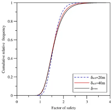
Fig. 11(b) and 12(b)show the probability distribu-tions of the factor of safety for two different scales of fluctuation along the failure. They show that the histogram of the factor of safety has positive skewness. This means it has a longer tail on the right than on the left. The coefficient of skewness, which is a measure of asymmetry in the distribution, increases with an increase
of the scale of fluctuation, as presented inTable 7. As
can be seen in the graph of cumulative probability in Fig. 13, the probability of failure increases as the coefficient of skewness increases.
6. Conclusions
This paper considered slope stability problems with uncertain quantities through a numerical procedure based on Monte Carlo simulations that consider the spatial variability of the soil properties. The approach adopts a first-order reliability method based on the stability model presented by Spencer in order to deter-mine the critical failure surface and to conduct a prelim-inary sensitivity analysis for the selective consideration of a few random parameters as random fields. Soil properties, represented as random fields, are then dis-cretized into sets of correlated random variables for use in the Monte Carlo simulation.
Probabilistic stability assessments were performed to obtain the variation of failure probability with variation of the soil parameters in layered slopes. The searched critical probabilistic surfaces showed somewhat differ-ent locations from the critical deterministic surface. The numerical examples also demonstrated that the correla-tion characteristics of the random field have a strong influence on the estimated failure probabilities and the convergence of the analysis.
Although the examples are limited to a two-dimensional random field, they provide insight into the application of uncertainty treatment to slope stability analyses and show the importance of the spatial vari-ability of soil properties in the outcome of a probabilistic assessment.
References
Alonso, E.E., 1976. Risk analysis of slopes and its application to slopes in Canadian sensitive clays. Geotechnique 26, 453–472.
Auvinet, G., González, J.L., 2000. Three-dimensional reliability analysis of earth slopes. Computers and Geotechnics 26, 247–261.
Baecher, G.B., Christian, J.T., 2003. Reliability and Statistics in Geotechnical Engineering. John Wiley & Sons.
Bhattacharya, G., Jana, D., Ojha, S., Chakraborty, S., 2003. Direct search for minimum reliability index of earth slopes. Computers and Geotechnics 30, 455–462.
Bolton, H.P.J., Heymann, G., Groenwold, A., 2003. Global search for critical failure surface in slope stability analysis. Engineering Optimization 35, 51–65.
Cheng, Y.M., 2003. Locations of critical failure surface and some further studies on slope stability analysis. Computers and Geotechnics 30, 255–267.
Chowdhury, R.N., Xu, D.W., 1995. Geotechnical system reliability of slopes. Reliability Engineering and Systems Safety 47, 141–151. Christian, J.T., Ladd, C.C., Baecher, G.B., 1994. Reliability applied to slope stability analysis. Journal of the Geotechnical Engineering Division, ASCE 120, 2180–2207.
D'Andrea, R., 2001. Discussion of“Search algorithm for minimum reliability index of earth slopes”by Hassan and Wolff. Journal of Geotechnical and Geoenvironmental Engineering, ASCE 127 (2), 195–197.
Elkateb, T., Chalaturnyk, R., Robertson, P.K., 2002. An overview of soil heterogeneity: quantification and implications on geotechnical field problems. Canadian Geotechnical Journal 40, 1–15. El-Ramly, H., Morgenstern, N.R., Cruden, D.M., 2002. Probabilistic
slope stability analysis for practice. Canadian Geotechnical Journal 39, 665–683.
El-Ramly, H., Morgenstern, N.R., Cruden, D.M., 2003. Probabilistic stability analysis of a tailings dyke on presheared clay-shale. Canadian Geotechnical Journal 40, 192–208.
Greco, V.R., 1996. Efficient Monte Carlo technique for locating critical slip surface. Journal of the Geotechnical Engineering Division, ASCE 122, 517–525.
Griffiths, D.V., Fenton, G.A., 2004. Probabilistic slope stability analysis by finite elements. Journal of the Geotechnical Engineer-ing Division, ASCE 130 (5), 507–518.
Hasofer, A.M., Lind, N.C., 1974. Exact and invariant second-moment code format. Journal of the Engineering Mechanics Division, ASCE 100, 111–121.
Hassan, A.M., Wolff, T.F., 1999. Search algorithm for minimum reliability index of earth slopes. Journal of the Geotechnical Engineering Division, ASCE 125, 301–308.
Haukaas, T., Der Kiuregian, A., 2001. A computer program for nonlinear finite element analysis. Proceedings of the Eighth Inter-national Conference on Structural Safety and Reliability, Newport Beach, CA.
Kim, J.Y., Lee, S.R., 1997. An improved search strategy for the critical slip surface using finite element stress fields. Computers and Geotechnics 21 (4), 295–313.
Knabe, W., Przewlocki, J., Rozynski, G., 1998. Spatial averages for linear elements for two-parameter random field. Probalistic Engineering Mechanics 13, 147–167.
Lacasse, S., Nadim, F., 1996. Uncertainties in characterizing soil properties. In: Shackleford, C.D., Nelson, P.P., Roth, M.J.S. (Eds.), Uncertainty in the Geologic Environment: From Theory to Practice. ASCE Geotechnical Special Publication, vol. 58, pp. 49–75. Li, K.S., Cheung, R.W.M., 2001. Discussion of“Search algorithm for
Li, K.S., Lumb, P., 1987. Probabilistic design of slopes. Canadian Geotechnical Journal 24, 520–535.
Li, K.S., White, W., 1987. Rapid evaluation of the critical slip surface in slope stability problem. International Journal for Numerical and Analytical Methods in Geomechanics 11, 449–473.
Liang, R.Y., Nusier, O.K., Malkawi, A.H., 1999. A reliability based approach for evaluating the slope stability of embankmen dams. Engineering Geology 54, 271–285.
Liu, P.L., Der Kiureghian, A., 1990. Optimization algorithms for structural reliability. Structural Safety 9, 161–177.
Low, B.K., 2003. Practical probabilistic slope stability analysis. 12th Panamerican Conference on Soil Mechanics and Geotechnical Engineering and 39th U.S. Rock Mechanics Symposium, vol. 2. MIT, Cambridge, Massachusetts, pp. 2777–2784.
Low, B.K., Tang, W.H., 1997. Reliability analysis of reinforced embankments on soft ground. Canadian Geotechnical Journal 34, 672–685.
Low, B.K., Gilbert, R.B., Wright, S.G., 1998. Slope reliability analysis using generalized method of slices. Journal of the Geotechnical Engineering Division, ASCE 124, 350–362.
Mostyn, G.R., Li, K.S., 1993. Probabilistic slope stability—state of play. In: Li, Lo (Eds.), Conf. on Probabilistic Methods in Geotechnical Engineering. Balkema, Rotterdam, The Netherlands, pp. 89–110.
Rackwitz, R., 2000. Reviewing probabilistic soils modeling. Compu-ters and Geotechnics 26, 199–223.
Rackwitz, R., Fiessler, B., 1978. Structural reliability under combined load sequences. Computers and Structures 9, 489–494.
Spencer, E., 1967. A method of analysis for stability of embankments using parallel inter-slice forces. Geotechnique 17 (1), 11–26. Stein, M.L., 1987. Large sample properties of simulations using Latin
hypercube sampling. Technometrics 29, 143–151.
US Army Corps Engineers, 1995. Introduction to probability and reliability methods for use in geotechnical engineering. Engineer-ing Technical Letter No. 1110-2-547. U.S. Arm Corps of Engineer, Department of the Army, Washington D.C.
Vanmarcke, E.H., 1977a. Probabilistic modeling of soil profiles. Journal of the Geotechnical Engineering Division, ASCE 103, 1227–1246.
Vanmarcke, E.H., 1977b. Reliability of earth slopes. Journal of the Geotechnical Engineering Division, ASCE 103, 1247–1265. Vanmarcke, E.H., 1983. Random Fields: Analysis and Synthesis. The
MIT Press, Cambridge, MA.