Business Series
The Wiley & SAS Business Series presents books that help senior‐level managers with their critical management decisions.
Titles in the Wiley & SAS Business Series include:
Activity‐Based Management for Financial Institutions: Driving Bottom‐ Line Results by Brent Bahnub
Bank Fraud: Using Technology to Combat Losses by Revathi Subramanian
Big Data Analytics: Turning Big Data into Big Money by Frank Ohlhorst
Branded! How Retailers Engage Consumers with Social Media and Mobil-ityby Bernie Brennan and Lori Schafer
Business Analytics for Customer Intelligence by Gert Laursen
Business Analytics for Managers: Taking Business Intelligence beyond Reporting by Gert Laursen and Jesper Thorlund
The Business Forecasting Deal: Exposing Bad Practices and Providing Practical Solutions by Michael Gilliland
Business Intelligence Applied: Implementing an Effective Information and Communications Technology Infrastructure by Michael Gendron
Business Intelligence in the Cloud: Strategic Implementation Guide by Michael S. Gendron
Business Intelligence Success Factors: Tools for Aligning Your Business in the Global Economy by Olivia Parr Rud
CIO Best Practices: Enabling Strategic Value with Information Technology, second edition by Joe Stenzel
Connecting Organizational Silos: Taking Knowledge Flow Management to the Next Level with Social Media by Frank Leistner
The Data Asset: How Smart Companies Govern Their Data for Business Success by Tony Fisher
Delivering Business Analytics: Practical Guidelines for Best Practice by Evan Stubbs
Demand‐Driven Forecasting: A Structured Approach to Forecasting, Sec-ond Edition by Charles Chase
Demand‐Driven Inventory Optimization and Replenishment: Creating a More Effi cient Supply Chain by Robert A. Davis
The Executive’s Guide to Enterprise Social Media Strategy: How Social Net-works Are Radically Transforming Your Business by David Thomas and Mike Barlow
Economic and Business Forecasting: Analyzing and Interpreting Econo-metric Results by John Silvia, Azhar Iqbal, Kaylyn Swankoski, Sarah Watt, and Sam Bullard
Executive’s Guide to Solvency II by David Buckham, Jason Wahl, andI Stuart Rose
Fair Lending Compliance: Intelligence and Implications for Credit Risk Management by Clark R. Abrahams and Mingyuan Zhangt
Foreign Currency Financial Reporting from Euros to Yen to Yuan: A Guide to Fundamental Concepts and Practical Applications by Robert Rowan
Health Analytics: Gaining the Insights to Transform Health Care by Jason Burke
Heuristics in Analytics: A Practical Perspective of What Infl uences Our Analytical World by Carlos Andre Reis Pinheiro and Fiona McNeilld
Human Capital Analytics: How to Harness the Potential of Your Organiza-tion’s Greatest Asset by Gene Pease, Boyce Byerly, and Jac Fitz‐enz t
Implement, Improve and Expand Your Statewide Longitudinal Data Sys-tem: Creating a Culture of Data in Education by Jamie McQuiggan and Armistead Sapp
Manufacturing Best Practices: Optimizing Productivity and Product Qual-ityby Bobby Hull
Marketing Automation: Practical Steps to More Effective Direct Marketing by Jeff LeSueur
Mastering Organizational Knowledge Flow: How to Make Knowledge Sharing Workby Frank Leistner
The New Know: Innovation Powered by Analytics by Thornton May
Performance Management: Integrating Strategy Execution, Methodologies, Risk, and Analytics by Gary Cokins
Predictive Business Analytics: Forward‐Looking Capabilities to Improve Business Performance by Lawrence Maisel and Gary Cokins
Retail Analytics: The Secret Weapon by Emmett Cox
Social Network Analysis in Telecommunications by Carlos Andre Reis Pinheiro
Statistical Thinking: Improving Business Performance, second edition by Roger W. Hoerl and Ronald D. Snee
Taming the Big Data Tidal Wave: Finding Opportunities in Huge Data Streams with Advanced Analytics by Bill Franks
Too Big to Ignore: The Business Case for Big Data by Phil Simon
The Value of Business Analytics: Identifying the Path to Profi tability by Evan Stubbs
Visual Six Sigma: Making Data Analysis Lean by Ian Cox, Marie A. Gaudard, Philip J. Ramsey, Mia L. Stephens, and Leo Wright
Win with Advanced Business Analytics: Creating Business Value from Your Data by Jean Paul Isson and Jesse Harriott
Analytics in a Big
Data World
The Essential Guide to Data Science
and Its Applications
Copyright © 2014 by Bart Baesens. All rights reserved.
Published by John Wiley & Sons, Inc., Hoboken, New Jersey. Published simultaneously in Canada.
No part of this publication may be reproduced, stored in a retrieval system, or transmitted in any form or by any means, electronic, mechanical, photocopying, recording, scanning, or otherwise, except as permitted under Section 107 or 108 of the 1976 United States Copyright Act, without either the prior written permission of the Publisher, or authorization through payment of the appropriate per-copy fee to the Copyright Clearance Center, Inc., 222 Rosewood Drive, Danvers, MA 01923, (978) 750-8400, fax (978) 646-8600, or on the Web at www.copyright.com. Requests to the Publisher for permission should be addressed to the Permissions Department, John Wiley & Sons, Inc., 111 River Street, Hoboken, NJ 07030, (201) 748-6011, fax (201) 748-6008, or online at http://www.wiley.com/go/permissions.
Limit of Liability/Disclaimer of Warranty: While the publisher and author have used their best efforts in preparing this book, they make no representations or warranties with respect to the accuracy or completeness of the contents of this book and specifi cally disclaim any implied warranties of merchantability or fi tness for a particular purpose. No warranty may be created or extended by sales representatives or written sales materials. The advice and strategies contained herein may not be suitable for your situation. You should consult with a professional where appropriate. Neither the publisher nor author shall be liable for any loss of profi t or any other commercial damages, including but not limited to special, incidental, consequential, or other damages.
For general information on our other products and services or for technical support, please contact our Customer Care Department within the United States at (800) 762-2974, outside the United States at (317) 572-3993 or fax (317) 572-4002.
Wiley publishes in a variety of print and electronic formats and by print-on-demand. Some material included with standard print versions of this book may not be included in e-books or in print-on-demand. If this book refers to media such as a CD or DVD that is not included in the version you purchased, you may download this material at http://booksupport.wiley.com. For more information about Wiley products, visit www.wiley.com.
Library of Congress Cataloging-in-Publication Data: Baesens, Bart.
Analytics in a big data world : the essential guide to data science and its applications / Bart Baesens.
1 online resource. — (Wiley & SAS business series)
Description based on print version record and CIP data provided by publisher; resource not viewed.
ISBN 978-1-118-89271-8 (ebk); ISBN 978-1-118-89274-9 (ebk);
ISBN 978-1-118-89270-1 (cloth) 1. Big data. 2. Management—Statistical methods. 3. Management—Data processing. 4. Decision making—Data processing. I. Title.
HD30.215 658.4’038 dc23
2014004728
Printed in the United States of America
ix
Preface xiii
Acknowledgments xv
Chapter 1 Big Data and Analytics 1 Example Applications 2
Basic Nomenclature 4 Analytics Process Model 4 Job Profi les Involved 6 Analytics 7
Analytical Model Requirements 9 Notes 10
Chapter 2 Data Collection, Sampling, and Preprocessing 13 Types of Data Sources 13
Sampling 15
Types of Data Elements 17
Visual Data Exploration and Exploratory Statistical Analysis 17
Missing Values 19
Outlier Detection and Treatment 20 Standardizing Data 24
Categorization 24
Segmentation 32 Notes 33
Chapter 3 Predictive Analytics 35 Target Defi nition 35
Linear Regression 38 Logistic Regression 39 Decision Trees 42 Neural Networks 48
Support Vector Machines 58 Ensemble Methods 64
Multiclass Classifi cation Techniques 67 Evaluating Predictive Models 71 Notes 84
Chapter 4 Descriptive Analytics 87 Association Rules 87
Sequence Rules 94 Segmentation 95 Notes 104
Chapter 5 Survival Analysis 105 Survival Analysis Measurements 106 Kaplan Meier Analysis 109
Parametric Survival Analysis 111 Proportional Hazards Regression 114 Extensions of Survival Analysis Models 116 Evaluating Survival Analysis Models 117 Notes 117
Chapter 6 Social Network Analytics 119 Social Network Defi nitions 119
Probabilistic Relational Neighbor Classifi er 125 Relational Logistic Regression 126
Collective Inferencing 128 Egonets 129
Bigraphs 130 Notes 132
Chapter 7 Analytics: Putting It All to Work 133 Backtesting Analytical Models 134
Benchmarking 146 Data Quality 149 Software 153 Privacy 155
Model Design and Documentation 158 Corporate Governance 159
Notes 159
Chapter 8 Example Applications 161 Credit Risk Modeling 161
Fraud Detection 165
Net Lift Response Modeling 168 Churn Prediction 172
Recommender Systems 176 Web Analytics 185
Social Media Analytics 195 Business Process Analytics 204 Notes 220
About the Author 223
xiii
C
ompanies are being fl ooded with tsunamis of data collected in a multichannel business environment, leaving an untapped poten-tial for analytics to better understand, manage, and strategically exploit the complex dynamics of customer behavior. In this book, we will discuss how analytics can be used to create strategic leverage and identify new business opportunities.The focus of this book is not on the mathematics or theory, but on the practical application. Formulas and equations will only be included when absolutely needed from a practitioner’s perspective. It is also not our aim to provide exhaustive coverage of all analytical techniques previously developed, but rather to cover the ones that really provide added value in a business setting.
The book is written in a condensed, focused way because it is tar-geted at the business professional. A reader’s prerequisite knowledge should consist of some basic exposure to descriptive statistics (e.g., mean, standard deviation, correlation, confi dence intervals, hypothesis testing), data handling (using, for example, Microsoft Excel, SQL, etc.), and data visualization (e.g., bar plots, pie charts, histograms, scatter plots). Throughout the book, many examples of real‐life case studies will be included in areas such as risk management, fraud detection, customer relationship management, web analytics, and so forth. The author will also integrate both his research and consulting experience throughout the various chapters. The book is aimed at senior data ana-lysts, consultants, analytics practitioners, and PhD researchers starting to explore the fi eld.
xv
I
would like to acknowledge all my colleagues who contributed to1
C H A P T E R
1
Big Data and
Analytics
D
ata are everywhere. IBM projects that every day we generate 2.5 quintillion bytes of data.1 In relative terms, this means 90 percent of the data in the world has been created in the last two years. Gartner projects that by 2015, 85 percent of Fortune 500 organizations will be unable to exploit big data for competitive advantage and about 4.4 million jobs will be created around big data. 2 Although these esti-mates should not be interpreted in an absolute sense, they are a strong indication of the ubiquity of big data and the strong need for analytical skills and resources because, as the data piles up, managing and analyz-ing these data resources in the most optimal way become critical suc-cess factors in creating competitive advantage and strategic leverage.exploit big data. In another poll ran by KDnuggets in July 2013, a strong need emerged for analytics/big data/data mining/data science educa-tion.4It is the purpose of this book to try and fi ll this gap by providing a
concise and focused overview of analytics for the business practitioner.
EXAMPLE APPLICATIONS
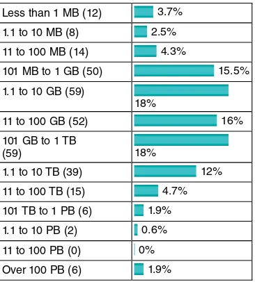
Analytics is everywhere and strongly embedded into our daily lives. As I am writing this part, I was the subject of various analytical models today. When I checked my physical mailbox this morning, I found a catalogue sent to me most probably as a result of a response modeling analytical exercise that indicated that, given my characteristics and previous pur-chase behavior, I am likely to buy one or more products from it. Today, I was the subject of a behavioral scoring model of my fi nancial institu-tion. This is a model that will look at, among other things, my check-ing account balance from the past 12 months and my credit payments during that period, together with other kinds of information available to my bank, to predict whether I will default on my loan during the next year. My bank needs to know this for provisioning purposes. Also today, my telephone services provider analyzed my calling behavior Figure 1.1 Results from a KDnuggets Poll about Largest Data Sets Analyzed
Source: www.kdnuggets.com/polls/2013/largest‐dataset‐analyzed‐data‐mined‐2013.html. Less than 1 MB (12) 3.7%
1.1 to 10 MB (8) 2.5%
11 to 100 MB (14) 4.3%
101 MB to 1 GB (50) 15.5%
1.1 to 10 GB (59)
18%
11 to 100 GB (52) 16%
101 GB to 1 TB
(59) 18%
1.1 to 10 TB (39) 12%
11 to 100 TB (15) 4.7%
101 TB to 1 PB (6) 1.9% 1.1 to 10 PB (2) 0.6%
11 to 100 PB (0) 0%
and my account information to predict whether I will churn during the next three months. As I logged on to my Facebook page, the social ads appearing there were based on analyzing all information (posts, pictures, my friends and their behavior, etc.) available to Facebook. My Twitter posts will be analyzed (possibly in real time) by social media analytics to understand both the subject of my tweets and the sentiment of them.
As I checked out in the supermarket, my loyalty card was scanned fi rst, followed by all my purchases. This will be used by my supermarket to analyze my market basket, which will help it decide on product bun-dling, next best offer, improving shelf organization, and so forth. As I made the payment with my credit card, my credit card provider used a fraud detection model to see whether it was a legitimate transaction. When I receive my credit card statement later, it will be accompanied by various vouchers that are the result of an analytical customer segmenta-tion exercise to better understand my expense behavior.
To summarize, the relevance, importance, and impact of analytics are now bigger than ever before and, given that more and more data are being collected and that there is strategic value in knowing what is hidden in data, analytics will continue to grow. Without claiming to be exhaustive, Table 1.1 presents some examples of how analytics is applied in various settings.
Table 1.1 Example Analytics Applications
Marketing
Risk
Management Government Web Logistics Other
Response modeling
Credit risk modeling
It is the purpose of this book to discuss the underlying techniques and key challenges to work out the applications shown in Table 1.1 using analytics. Some of these applications will be discussed in further detail in Chapter 8 .
BASIC NOMENCLATURE
In order to start doing analytics, some basic vocabulary needs to be
defi ned. A fi rst important concept here concerns the basic unit of anal-ysis. Customers can be considered from various perspectives. Customer lifetime value (CLV) can be measured for either individual customers or at the household level. Another alternative is to look at account behavior. For example, consider a credit scoring exercise for which the aim is to predict whether the applicant will default on a particular mortgage loan account. The analysis can also be done at the transac-tion level. For example, in insurance fraud detectransac-tion, one usually per-forms the analysis at insurance claim level. Also, in web analytics, the basic unit of analysis is usually a web visit or session.
It is also important to note that customers can play different roles. For example, parents can buy goods for their kids, such that there is a clear distinction between the payer and the end user. In a banking setting, a customer can be primary account owner, secondary account owner, main debtor of the credit, codebtor, guarantor, and so on. It is very important to clearly distinguish between those different roles when defi ning and/or aggregating data for the analytics exercise.
Finally, in case of predictive analytics, the target variable needs to be appropriately defi ned. For example, when is a customer considered to be a churner or not, a fraudster or not, a responder or not, or how should the CLV be appropriately defi ned?
ANALYTICS PROCESS MODEL
data will have a deterministic impact on the analytical models that will be built in a subsequent step. All data will then be gathered in a stag-ing area, which could be, for example, a data mart or data warehouse. Some basic exploratory analysis can be considered here using, for example, online analytical processing (OLAP) facilities for
multidimen-sional data analysis (e.g., roll‐up, drill down, slicing and dicing). This will be followed by a data cleaning step to get rid of all inconsistencies, such as missing values, outliers, and duplicate data. Additional trans-formations may also be considered, such as binning, alphanumeric to numeric coding, geographical aggregation, and so forth. In the analyt-ics step, an analytical model will be estimated on the preprocessed and transformed data. Different types of analytics can be considered here (e.g., to do churn prediction, fraud detection, customer segmentation, market basket analysis). Finally, once the model has been built, it will be interpreted and evaluated by the business experts. Usually, many trivial patterns will be detected by the model. For example, in a market basket analysis setting, one may fi nd that spaghetti and spaghetti sauce are often purchased together. These patterns are interesting because they provide some validation of the model. But of course, the key issue here is to fi nd the unexpected yet interesting and actionable patterns (sometimes also referred to as knowledge diamonds ) that can provide added value in the business setting. Once the analytical model has been appropriately validated and approved, it can be put into produc-tion as an analytics applicaproduc-tion (e.g., decision support system, scoring engine). It is important to consider here how to represent the model output in a user‐friendly way, how to integrate it with other applica-tions (e.g., campaign management tools, risk engines), and how to make sure the analytical model can be appropriately monitored and backtested on an ongoing basis.
JOB PROFILES INVOLVED
Analytics is essentially a multidisciplinary exercise in which many different job profi les need to collaborate together. In what follows, we will discuss the most important job profi les.
The database or data warehouse administrator (DBA) is aware of all the data available within the fi rm, the storage details, and the data defi nitions. Hence, the DBA plays a crucial role in feeding the analyti-cal modeling exercise with its key ingredient, which is data. Because analytics is an iterative exercise, the DBA may continue to play an important role as the modeling exercise proceeds.
Another very important profi le is the business expert. This could, for example, be a credit portfolio manager, fraud detection expert, brand manager, or e‐commerce manager. This person has extensive business experience and business common sense, which is very valu-able. It is precisely this knowledge that will help to steer the analytical modeling exercise and interpret its key fi ndings. A key challenge here is that much of the expert knowledge is tacit and may be hard to elicit at the start of the modeling exercise.
Legal experts are becoming more and more important given that not all data can be used in an analytical model because of privacy, Figure 1.2 The Analytics Process Model
Understanding what data is needed for the application
Data Cleaning
Interpretation and Evaluation
Data Transformation (binning, alpha to numeric, etc.)
Analytics
Data Selection
Source Data
Analytics Application
Preprocessed Data
Transformed Data
Patterns
Data Mining Mart
discrimination, and so forth. For example, in credit risk modeling, one can typically not discriminate good and bad customers based upon gender, national origin, or religion. In web analytics, information is
typically gathered by means of cookies, which are fi les that are stored on the user’s browsing computer. However, when gathering informa-tion using cookies, users should be appropriately informed. This is sub-ject to regulation at various levels (both national and, for example, European). A key challenge here is that privacy and other regulation highly vary depending on the geographical region. Hence, the legal expert should have good knowledge about what data can be used when, and what regulation applies in what location.
The data scientist, data miner, or data analyst is the person respon-sible for doing the actual analytics. This person should possess a thor-ough understanding of all techniques involved and know how to implement them using the appropriate software. A good data scientist should also have good communication and presentation skills to report the analytical fi ndings back to the other parties involved.
The software tool vendors should also be mentioned as an important part of the analytics team. Different types of tool vendors can be distinguished here. Some vendors only provide tools to automate specifi c steps of the analytical modeling process (e.g., data preprocess-ing). Others sell software that covers the entire analytical modeling process. Some vendors also provide analytics‐based solutions for spe-cifi c application areas, such as risk management, marketing analytics and campaign management, and so on.
ANALYTICS
Analytics is a term that is often used interchangeably with data science, data mining, knowledge discovery, and others. The distinction between all those is not clear cut. All of these terms essentially refer to extract-ing useful business patterns or mathematical decision models from a preprocessed data set. Different underlying techniques can be used for this purpose, stemming from a variety of different disciplines, such as:
■ Biology (e.g., neural networks, genetic algorithms, swarm intel-ligence)
■ Kernel methods (e.g., support vector machines)
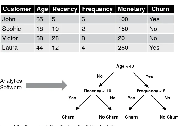
Basically, a distinction can be made between predictive and descrip-tive analytics. In predicdescrip-tive analytics, a target variable is typically avail-able, which can either be categorical (e.g., churn or not, fraud or not) or continuous (e.g., customer lifetime value, loss given default). In descriptive analytics, no such target variable is available. Common examples here are association rules, sequence rules, and clustering. Figure 1.3 provides an example of a decision tree in a classifi cation predictive analytics setting for predicting churn.
More than ever before, analytical models steer the strategic risk decisions of companies. For example, in a bank setting, the mini-mum equity and provisions a fi nancial institution holds are directly determined by, among other things, credit risk analytics, market risk analytics, operational risk analytics, fraud analytics, and insurance risk analytics. In this setting, analytical model errors directly affect profi tability, solvency, shareholder value, the macroeconomy, and society as a whole. Hence, it is of the utmost importance that analytical
Figure 1.3 Example of Classifi cation Predictive Analytics
Customer Age Recency Frequency Monetary Churn
John 35 5 6 100 Yes
Sophie 18 10 2 150 No
Victor 38 28 8 20 No
Laura 44 12 4 280 Yes
Analytics Software
Age < 40
Yes
Yes
Churn No Churn Churn No Churn
Yes No
No No
models are developed in the most optimal way, taking into account various requirements that will be discussed in what follows.
ANALYTICAL MODEL REQUIREMENTS
A good analytical model should satisfy several requirements,
depend-ing on the application area. A fi rst critical success factor is business relevance. The analytical model should actually solve the business problem for which it was developed. It makes no sense to have a work-ing analytical model that got sidetracked from the original problem statement. In order to achieve business relevance, it is of key impor-tance that the business problem to be solved is appropriately defi ned, qualifi ed, and agreed upon by all parties involved at the outset of the analysis.
A second criterion is statistical performance. The model should have statistical signifi cance and predictive power. How this can be mea-sured will depend upon the type of analytics considered. For example, in a classifi cation setting (churn, fraud), the model should have good discrimination power. In a clustering setting, the clusters should be as homogenous as possible. In later chapters, we will extensively discuss various measures to quantify this.
analytical models are incomprehensible and black box in nature. A popular example of this is neural networks, which are universal approximators and are high performing, but offer no insight into the underlying patterns in the data. On the contrary, linear regression models are very transparent and comprehensible, but offer only limited modeling power.
Analytical models should also be operationally effi cientt. This refers to the efforts needed to collect the data, preprocess it, evaluate the model, and feed its outputs to the business application (e.g., campaign man-agement, capital calculation). Especially in a real‐time online scoring environment (e.g., fraud detection) this may be a crucial characteristic. Operational effi ciency also entails the efforts needed to monitor and backtest the model, and reestimate it when necessary.
Another key attention point is the economic costt needed to set up the analytical model. This includes the costs to gather and preprocess the data, the costs to analyze the data, and the costs to put the result-ing analytical models into production. In addition, the software costs and human and computing resources should be taken into account here. It is important to do a thorough cost–benefi t analysis at the start of the project.
Finally, analytical models should also comply with both local and international regulation and legislation . For example, in a credit risk set-ting, the Basel II and Basel III Capital Accords have been introduced to appropriately identify the types of data that can or cannot be used to build credit risk models. In an insurance setting, the Solvency II Accord plays a similar role. Given the importance of analytics nowa-days, more and more regulation is being introduced relating to the development and use of the analytical models. In addition, in the con-text of privacy, many new regulatory developments are taking place at various levels. A popular example here concerns the use of cookies in a web analytics context.
NOTES
1. IBM, www.ibm.com/big‐data/us/en , 2013. 2. www.gartner.com/technology/topics/big‐data.jsp .
5. J. Han and M. Kamber, Data Mining: Concepts and Techniques, 2nd ed. (Morgan Kaufmann, Waltham, MA, US, 2006); D. J. Hand, H. Mannila, and P. Smyth, Prin-ciples of Data Mining (MIT Press, Cambridge , Massachusetts, London, England, 2001); P. N. Tan, M. Steinbach, and V. Kumar, Introduction to Data Mining (Pearson, Upper Saddle River, New Jersey, US, 2006).
13
C H A P T E R
2
Data Collection,
Sampling, and
Preprocessing
D
ata are key ingredients for any analytical exercise. Hence, it is important to thoroughly consider and list all data sources that are of potential interest before starting the analysis. The rule here is the more data, the better. However, real life data can be dirty because of inconsistencies, incompleteness, duplication, and merging problems. Throughout the analytical modeling steps, various data fi ltering mecha-nisms will be applied to clean up and reduce the data to a manageable and relevant size. Worth mentioning here is the garbage in, garbage out (GIGO) principle, which essentially states that messy data will yield messy analytical models. It is of the utmost importance that every data preprocessing step is carefully justifi ed, carried out, validated, and doc-umented before proceeding with further analysis. Even the slightest mistake can make the data totally unusable for further analysis. In what follows, we will elaborate on the most important data preprocessing steps that should be considered during an analytical modeling exercise.TYPES OF DATA SOURCES
Transactions are the fi rst important source of data. Transactional data consist of structured, low‐level, detailed information capturing the key characteristics of a customer transaction (e.g., purchase, claim, cash transfer, credit card payment). This type of data is usually stored in massive online transaction processing (OLTP) relational databases. It can also be summarized over longer time horizons by aggregating it into averages, absolute/relative trends, maximum/minimum values, and so on.
Unstructured data embedded in text documents (e.g., emails, web pages, claim forms) or multimedia content can also be interesting to analyze. However, these sources typically require extensive preprocess-ing before they can be successfully included in an analytical exercise. Another important source of data is qualitative, expert‐based data. An expert is a person with a substantial amount of subject mat-ter expertise within a particular setting (e.g., credit portfolio manager, brand manager). The expertise stems from both common sense and business experience, and it is important to elicit expertise as much as possible before the analytics is run. This will steer the modeling in the right direction and allow you to interpret the analytical results from the right perspective. A popular example of applying expert‐based validation is checking the univariate signs of a regression model. For example, one would expect a priorii that higher debt has an adverse impact on credit risk, such that it should have a negative sign in the fi nal scorecard. If this turns out not to be the case (e.g., due to bad data quality, multicollinearity), the expert/business user will not be tempted to use the analytical model at all, since it contradicts prior expectations.
as their fi nal internal model, or as a benchmark against an internally developed credit scorecard to better understand the weaknesses of the latter.
Finally, plenty of publicly available data can be included in the analytical exercise. A fi rst important example is macroeconomic data about gross domestic product (GDP), infl ation, unemployment, and so on. By including this type of data in an analytical model, it will become possible to see how the model varies with the state of the economy. This is especially relevant in a credit risk setting, where typically all models need to be thoroughly stress tested. In addition, social media data from Facebook, Twitter, and others can be an important source of information. However, one needs to be careful here and make sure that all data gathering respects both local and international privacy regulations.
SAMPLING
The aim of sampling is to take a subset of past customer data and use that to build an analytical model. A fi rst obvious question concerns the need for sampling. With the availability of high performance comput-ing facilities (e.g., grid/cloud computcomput-ing), one could also directly ana-lyze the full data set. However, a key requirement for a good sample is that it should be representative of the future customers on which the analytical model will be run. Hence, the timing aspect becomes important because customers of today are more similar to customers of tomorrow than customers of yesterday. Choosing the optimal time window for the sample involves a trade‐off between lots of data (and hence a more robust analytical model) and recent data (which may be more representative). The sample should also be taken from an aver-age business period to get a picture of the target population that is as accurate as possible.
then needs a subset of the historical TTD population to build an ana-lytical model. However, in the past, the bank was already applying a credit policy (either expert based or based on a previous analytical model). This implies that the historical TTD population has two subsets: the customers that were accepted with the old policy, and the ones that were rejected (see Figure 2.1 ). Obviously, for the latter, we don’t know the target value since they were never granted the credit. When build-ing a sample, one can then only make use of those that were accepted, which clearly implies a bias. Procedures for reject inference have been suggested in the literature to deal with this sampling bias problem. 1 Unfortunately, all of these procedures make assumptions and none of them works perfectly. One of the most popular solutions is bureau‐ based inference, whereby a sample of past customers is given to the credit bureau to determine their target label (good or bad payer).
When thinking even closer about the target population for credit scoring, another forgotten subset are the withdrawals. These are the customers who were offered credit but decided not to take it (despite the fact that they may have been classifi ed as good by the old scorecard). To be representative, these customers should also be included in the development sample. However, to the best of our knowledge, no procedures for withdrawal inference are typically applied in the industry.
In stratifi ed sampling, a sample is taken according to predefi ned strata. Consider, for example, a churn prediction or fraud detection context in which data sets are typically very skewed (e.g., 99 percent nonchurners and 1 percent churners). When stratifying according to the target churn indicator, the sample will contain exactly the same percentages of churners and nonchurners as in the original data. Figure 2.1 The Reject Inference Problem in Credit Scoring
Through-the-Door
Rejects Accepts
Bads Goods
TYPES OF DATA ELEMENTS
It is important to appropriately consider the different types of data ele-ments at the start of the analysis. The following types of data eleele-ments can be considered:
■ Continuous: These are data elements that are defi ned on an
interval that can be limited or unlimited. Examples include income, sales, RFM (recency, frequency, monetary).
■ Categorical
■ Nominal: These are data elements that can only take on a
limited set of values with no meaningful ordering in between. Examples include marital status, profession, purpose of loan.
■ Ordinal: These are data elements that can only take on a
lim-ited set of values with a meaningful ordering in between. Examples include credit rating; age coded as young, middle aged, and old.
■ Binary: These are data elements that can only take on two
values. Examples include gender, employment status.
Appropriately distinguishing between these different data elements is of key importance to start the analysis when importing the data into an analytics tool. For example, if marital status were to be incor-rectly specifi ed as a continuous data element, then the software would calculate its mean, standard deviation, and so on, which is obviously meaningless.
VISUAL DATA EXPLORATION AND EXPLORATORY STATISTICAL ANALYSIS
for free (e.g., live with parents). By doing a separate pie chart analysis for the goods and bads, respectively, one can see that more goods own their residential property than bads, which can be a very useful start-ing insight. Bar charts represent the frequency of each of the values (either absolute or relative) as bars. Other handy visual tools are histo-grams and scatter plots. A histogram provides an easy way to visualize the central tendency and to determine the variability or spread of the data. It also allows you to contrast the observed data with standard known distributions (e.g., normal distribution). Scatter plots allow you to visualize one variable against another to see whether there are any correlation patterns in the data. Also, OLAP‐based multidimensional data analysis can be usefully adopted to explore patterns in the data.
A next step after visual analysis could be inspecting some basic statistical measurements, such as averages, standard deviations, mini-mum, maximini-mum, percentiles, and confi dence intervals. One could calculate these measures separately for each of the target classes Figure 2.2 Pie Charts for Exploratory Data Analysis
Total Population
Own Rent For Free
Goods
Own Rent For Free
Bads
(e.g., good versus bad customer) to see whether there are any interest-ing patterns present (e.g., whether bad payers usually have a lower average age than good payers).
MISSING VALUES
Missing values can occur because of various reasons. The information can be nonapplicable. For example, when modeling time of churn, this information is only available for the churners and not for the non-churners because it is not applicable there. The information can also be undisclosed. For example, a customer decided not to disclose his or her income because of privacy. Missing data can also originate because of an error during merging (e.g., typos in name or ID).
Some analytical techniques (e.g., decision trees) can directly deal with missing values. Other techniques need some additional prepro-cessing. The following are the most popular schemes to deal with miss-ing values: 2
■ Replace (impute). This implies replacing the missing value with a known value (e.g., consider the example in Table 2.1 ). One could impute the missing credit bureau scores with the average or median of the known values. For marital status, the mode can then be used. One could also apply regression‐based imputation whereby a regression model is estimated to model a target variable (e.g., credit bureau score) based on the other information available (e.g., age, income). The latter is more sophisticated, although the added value from an empirical view-point (e.g., in terms of model performance) is questionable.
■ Delete. This is the most straightforward option and consists of
deleting observations or variables with lots of missing values. This, of course, assumes that information is missing at random and has no meaningful interpretation and/or relationship to the target.
■ Keep. Missing values can be meaningful (e.g., a customer did
As a practical way of working, one can fi rst start with statistically testing whether missing information is related to the target variable (using, for example, a chi‐squared test, discussed later). If yes, then we can adopt the keep strategy and make a special category for it. If not, one can, depending on the number of observations available, decide to either delete or impute.
OUTLIER DETECTION AND TREATMENT
Outliers are extreme observations that are very dissimilar to the rest of the population. Actually, two types of outliers can be considered:
1. Valid observations (e.g., salary of boss is $1 million)
2. Invalid observations (e.g., age is 300 years)
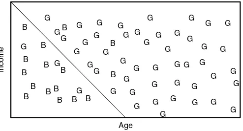
Both are univariate outliers in the sense that they are outlying on one dimension. However, outliers can be hidden in unidimensional views of the data. Multivariate outliers are observations that are ing in multiple dimensions. Figure 2.3 gives an example of two outly-ing observations consideroutly-ing both the dimensions of income and age.
Two important steps in dealing with outliers are detection and treat-ment. A fi rst obvious check for outliers is to calculate the minimum and maximum values for each of the data elements. Various graphical Table 2.1 Dealing with Missing Values
ID Age Income
Marital Status
Credit Bureau
Score Class
1 34 1,800 ? 620 Churner
2 28 1,200 Single ? Nonchurner
3 22 1,000 Single ? Nonchurner
4 60 2,200 Widowed 700 Churner
5 58 2,000 Married ? Nonchurner
6 44 ? ? ? Nonchurner
7 22 1,200 Single ? Nonchurner
8 26 1,500 Married 350 Nonchurner
9 34 ? Single ? Churner
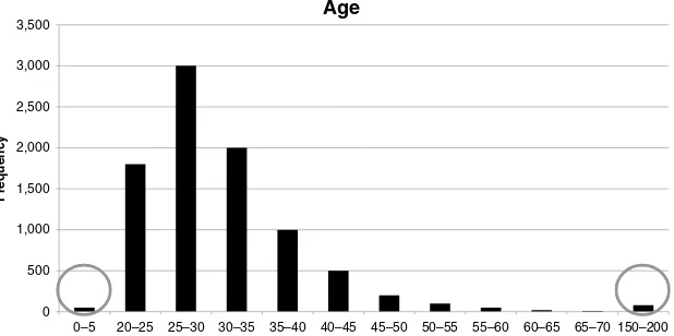
tools can be used to detect outliers. Histograms are a fi rst example. Figure 2.4 presents an example of a distribution for age whereby the circled areas clearly represent outliers.
Another useful visual mechanism are box plots. A box plot repre-sents three key quartiles of the data: the fi rst quartile (25 percent of the observations have a lower value), the median (50 percent of the observations have a lower value), and the third quartile (75 percent of the observations have a lower value). All three quartiles are rep-resented as a box. The minimum and maximum values are then also Figure 2.3 Multivariate Outliers
0 500 1,000 1,500 2,000 2,500 3,000 3,500 4,000 4,500
10 20 30 40 50 60 70
Income and Age
Figure 2.4 Histograms for Outlier Detection
0 500 1,000 1,500 2,000 2,500 3,000 3,500
0–5 20–25 25–30 30–35 35–40 40–45 45–50 50–55 55–60 60–65 65–70 150–200
Age
added unless they are too far away from the edges of the box. Too
far away is then quantifi ed as more than 1.5 * Interquartile Range (IQR = Q 3 − Q1 ). Figure 2.5 gives an example of a box plot in which three outliers can be seen.
Another way is to calculate z‐scores, measuring how many stan-dard deviations an observation lies away from the mean, as follows:
= − µ
σ
zi xi
where μ represents the average of the variable andσ its standard devi-ation. An example is given in Table 2.2 . Note that by defi nition, the
z ‐scores will have 0 mean and unit standard deviation.
z
A practical rule of thumb then defi nes outliers when the absolute value of the zz‐score |z| is bigger than 3. Note that the zz ‐score relies on the normal distribution.
The above methods all focus on univariate outliers. Multivariate outliers can be detected by fi tting regression lines and inspecting the
Table 2.2 Z‐Scores for Outlier Detection
ID Age Z ‐Score
1 30 (30 − 40)/10 = −1
2 50 (50 − 40)/10 = +1
3 10 (10 − 40)/10 = −3
4 40 (40 − 40)/10 = 0
5 60 (60 − 40)/10 = +2
6 80 (80 − 40)/10 = +4
… … …
μ μ= 40
σ= 10
μ μ= 0
σ= 1 Figure 2.5 Box Plots for Outlier Detection
Min Q1 M Q3
1.5 * IQR
observations with large errors (using, for example, a residual plot). Alternative methods are clustering or calculating the Mahalanobis dis-tance. Note, however, that although potentially useful, multivariate outlier detection is typically not considered in many modeling exer-cises due to the typical marginal impact on model performance.
Some analytical techniques (e.g., decision trees, neural net-works, Support Vector Machines (SVMs)) are fairly robust with respect to outliers. Others (e.g., linear/logistic regression) are more sensitive to them. Various schemes exist to deal with outliers. It highly depends on whether the outlier represents a valid or invalid observation. For invalid observations (e.g., age is 300 years), one could treat the outlier as a missing value using any of the schemes discussed in the previous section. For valid observations (e.g., income is $1 million), other schemes are needed. A popular scheme is truncation/capping/winsorizing. One hereby imposes both a lower and upper limit on a variable and any values below/above are brought back to these limits. The limits can be calculated using the zz‐scores (see Figure 2.6 ), or the IQR (which is more robust than the zz ‐scores), as follows:
Upper/lower limit=M 3s, with M± =median and s=IQR/(2 0.6745).× 3
A sigmoid transformation ranging between 0 and 1 can also be used for capping, as follows:
=
+ −
f x
e x
( ) 1
1
μ + 3σ
μ – 3σ μ
In addition, expert‐based limits based on business knowledge and/ or experience can be imposed.
STANDARDIZING DATA
Standardizing data is a data preprocessing activity targeted at scaling variables to a similar range. Consider, for example, two variables: gen-der (coded as 0/1) and income (ranging between $0 and $1 million). When building logistic regression models using both information ele-ments, the coeffi cient for income might become very small. Hence, it could make sense to bring them back to a similar scale. The following standardization procedures could be adopted:
■ Min/max standardization
■ = −
− − +
X X X
X X newmax newmin newmin
new old old
old old
min( )
max( ) min( )( ) ,
whereby newmax and newmin are the newly imposed maxi-mum and minimaxi-mum (e.g., 1 and 0).
■ ZZ ‐score standardization
■ Calculate the zz ‐scores (see the previous section) ■ Decimal scaling
■ Dividing by a power of 10 as follows: Xnew= Xoldn
10 , with n the number of digits of the maximum absolute value.
Again note that standardization is especially useful for regression‐ based approaches, but is not needed for decision trees, for example.
CATEGORIZATION
that fewer parameters will have to be estimated and a more robust model is obtained.
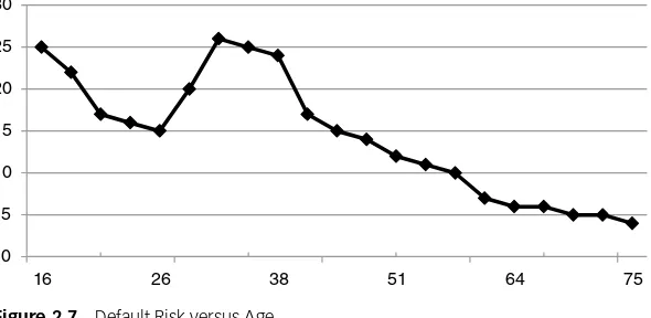
For continuous variables, categorization may also be very benefi -cial. Consider, for example, the age variable and its risk as depicted in Figure 2.7 . Clearly, there is a nonmonotonous relation between risk and age. If a nonlinear model (e.g., neural network, support vector machine) were to be used, then the nonlinearity can be perfectly mod-eled. However, if a regression model were to be used (which is typi-cally more common because of its interpretability), then since it can only fi t a line, it will miss out on the nonmonotonicity. By categorizing the variable into ranges, part of the nonmonotonicity can be taken into account in the regression. Hence, categorization of continuous variables can be useful to model nonlinear effects into linear models.
Various methods can be used to do categorization. Two very basic methods are equal interval binning and equal frequency binning. Consider, for example, the income values 1,000, 1,200, 1,300, 2,000, 1,800, and 1,400. Equal interval binning would create two bins with the same range—Bin 1: 1,000, 1,500 and Bin 2: 1,500, 2,000—whereas equal frequency binning would create two bins with the same num-ber of observations—Bin 1: 1,000, 1,200, 1,300; Bin 2: 1,400, 1,800, 2,000. However, both methods are quite basic and do not take into account a target variable (e.g., churn, fraud, credit risk).
Chi‐squared analysis is a more sophisticated way to do coarse sifi cation. Consider the example depicted in Table 2.3 for coarse clas-sifying a residential status variable.
0 5 10 15 20 25 30
16 26 38 51 64 75
Suppose we want three categories and consider the following options:
■ Option 1: owner, renters, others ■ Option 2: owner, with parents, others
Both options can now be investigated using chi‐squared analysis. The purpose is to compare the empirically observed with the indepen-dence frequencies. For option 1, the empirically observed frequencies are depicted in Table 2.4 .
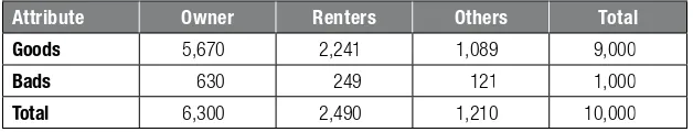
The independence frequencies can be calculated as follows. The number of good owners, given that the odds are the same as in the whole population, is 6,300/10,000 × 9,000/10,000 × 10,000 = 5,670. One then obtains Table 2.5 .
The more the numbers in both tables differ, the less independence, hence better dependence and a better coarse classifi cation. Formally, one can calculate the chi‐squared distance as follows:
χ = − + − + − + −
Table 2.3 Coarse Classifying the Residential Status Variable
Attribute Owner
6,000 1,600 350 950 90 10 9,000
Bads 300 400 140 100 50 10 1,000
Good: bad odds
20:1 4:1 2.5:1 9.5:1 1.8:1 1:1 9:1
Source: L. C. Thomas, D. Edelman, and J. N. Crook, Credit Scoring and its Applicationss (Society for Industrial and Applied Mathematics, Philadelphia, Penn., 2002).
Table 2.4 Empirical Frequencies Option 1 for Coarse Classifying Residential Status
Attribute Owner Renters Others Total
Goods 6,000 1,950 1,050 9,000
Bads 300 540 160 1,000
Table 2.5 Independence Frequencies Option 1 for Coarse Classifying Residential Status
Attribute Owner Renters Others Total
Goods 5,670 2,241 1,089 9,000
Bads 630 249 121 1,000
Total 6,300 2,490 1,210 10,000
Table 2.6 Coarse Classifying the Purpose Variable
Customer ID Age Purpose … G/B
C1 44 Car G
C2 20 Cash G
C3 58 Travel B
C4 26 Car G
C5 30 Study B
C6 32 House G
C7 48 Cash B
C8 60 Car G
… … …
Likewise, for option 2, the calculation becomes:
χ = − + − + − + −
+ − + − =
(6000 5670) 5670
(300 630) 630
(950 945) 945
(100 105) 105 (2050 2385)
2385
(600 265)
265 662
2 2 2 2 2
2 2
So, based upon the chi‐squared values, option 2 is the better cat-egorization. Note that formally, one needs to compare the value with a chi‐squared distribution with k − 1 degrees of freedom with k being the number of values of the characteristic.
Many analytics software tools have built‐in facilities to do catego-rization using chi‐squared analysis. A very handy and simple approach (available in Microsoft Excel) is pivot tables. Consider the example shown in Table 2.6 .
We can then categorize the values based on similar odds. For example, category 1 (car, study), category 2 (house), and category 3 (cash, travel).
WEIGHTS OF EVIDENCE CODING
Categorization reduces the number of categories for categorical vari-ables. For continuous variables, categorization will introduce new variables. Consider a regression model with age (4 categories, so 3 parameters) and purpose (5 categories, so 4 parameters) characteris-tics. The model then looks as follows:
Y Age Age Age Purp
Purp Purp Purp
0 1 1 2 2 3 3 4 1
5 2 6 3 7 4
= β + β + β + β + β
+ β + β + β
Despite having only two characteristics, the model still needs 8 parameters to be estimated. It would be handy to have a monotonic transformation f (.) such that our model could be rewritten as follows:ff
= β + β + β
Y 0 1f(Age , Age , Age )1 2 3 2f(Purp , Purp , Purp , Purp )1 2 3 4
The transformation should have a monotonically increasing or decreasing relationship with Y. Weights‐of‐evidence coding is one example of a transformation that can be used for this purpose. This is illustrated in Table 2.8 .
The WOE is calculated as: ln(Distr. Good/Distr. Bad). Because of the logarithmic transformation, a positive (negative) WOE means Distr. Good > (<) Distr. Bad. The WOE transformation thus imple-ments a transformation monotonically related to the target variable.
The model can then be reformulated as follows:
Y = β + β0 1WOEage+ β2WOEpurpose Table 2.7 Pivot Table for Coarse Classifying the Purpose Variable
Car Cash Travel Study House …
Good 1,000 2,000 3,000 100 5,000
Bad 500 100 200 80 800
This gives a more concise model than the model with which we started this section. However, note that the interpretability of the model becomes somewhat less straightforward when WOE variables are being used.
VARIABLE SELECTION
Many analytical modeling exercises start with tons of variables, of which typically only a few actually contribute to the prediction of the target variable. For example, the average application/behavioral scorecard in credit scoring has somewhere between 10 and 15 vari-ables. The key question is how to fi nd these variables. Filters are a very handy variable selection mechanism. They work by measuring univariate correlations between each variable and the target. As such, they allow for a quick screening of which variables should be retained for further analysis. Various fi lter measures have been suggested in the literature. One can categorize them as depicted in Table 2.9.
The Pearson correlationρPis calculated as follows:
∑
varies between −1 and +1. To apply it as a fi lter, one could select all variables for which the Pearson correlation is signifi cantly different Table 2.8 Calculating Weights of Evidence (WOE)
Age Count
18–22 200 10.00% 152 8.42% 48 24.74% −107.83%
23–26 300 15.00% 246 13.62% 54 27.84% −71.47%
27–29 450 22.50% 405 22.43% 45 23.20% −3.38%
30–35 500 25.00% 475 26.30% 25 12.89% 71.34%
35–44 350 17.50% 339 18.77% 11 5.67% 119.71%
44+ 150 7.50% 147 8.14% 3 1.55% 166.08%
from 0 (according to the p ‐value), or, for example, the ones where |ρP| > 0.50.
The Fisher score can be calculated as follows:
− the Fisher score indicate a predictive variable. To apply it as a fi lter, one could, for example, keep the top 10 percent. Note that the Fisher score may generalize to a well‐known analysis of variance (ANOVA) in case a variable has multiple categories.
The information value (IV) fi lter is based on weights of evidence and is calculated as follows:
∑
k represents the number of categories of the variable. For the
k
example discussed in Table 2.8 , the calculation becomes as depicted in Table 2.10 .
The following rules of thumb apply for the information value:
■ < 0.02: unpredictive ■ 0.02–0.1: weak predictive ■ 0.1–0.3: medium predictive ■ > 0.3: strong predictive
Note that the information value assumes that the variable has been categorized. It can actually also be used to adjust/steer the cat-egorization so as to optimize the IV. Many software tools will provide Table 2.9 Filters for Variable Selection
Continuous Target (e.g., CLV, LGD)
Categorical Target (e.g., churn, fraud, credit risk)
Continuous variable Pearson correlation Fisher score
interactive support to do this, whereby the modeler can adjust the categories and gauge the impact on the IV. To apply it as a fi lter, one can calculate the information value of all (categorical) variables and only keep those for which the IV > 0.1 or, for example, the top 10%.
Another fi lter measure based upon chi‐squared analysis is Cramer’s V. Consider the contingency table depicted in Table 2.11 for marital status versus good/bad.
Similar to the example discussed in the section on categorization, the chi‐squared value for independence can then be calculated as follows:
χ =(500 480)− + − + − + − =
480
(100 120) 120
(300 320) 320
(100 80)
80 10.41
2 2 2 2 2
k − 1 degrees of free-dom, with k being the number of classes of the characteristic. The Cramer’s V measure can then be calculated as follows:
Cramer s V
n 0.10,
2
′ = χ =
Table 2.10 Calculating the Information Value Filter Measure
Age Count
Distr.
Count Goods
Distr.
Good Bads
Distr.
Bad WOE IV
Missing 50 2.50% 42 2.33% 8 4.12% −57.28% 0.0103
18–22 200 10.00% 152 8.42% 48 24.74% −107.83% 0.1760
23–26 300 15.00% 246 13.62% 54 27.84% −71.47% 0.1016
27–29 450 22.50% 405 22.43% 45 23.20% −3.38% 0.0003
30–35 500 25.00% 475 26.30% 25 12.89% 71.34% 0.0957
35–44 350 17.50% 339 18.77% 11 5.67% 119.71% 0.1568
44+ 150 7.50% 147 8.14% 3 1.55% 166.08% 0.1095
Information Value 0.6502
Table 2.11 Contingency Table for Marital Status versus Good/Bad Customer
Good Bad Total
Married 500 100 600
Not Married 300 100 400
with n being the number of observations in the data set. Cramer’s V is always bounded between 0 and 1 and higher values indicate bet-ter predictive power. As a rule of thumb, a cutoff of 0.1 is commonly adopted. One can then again select all variables where Cramer’s V is bigger than 0.1, or consider the top 10 percent. Note that the informa-tion value and Cramer’s V typically consider the same characteristics as most important.
Filters are very handy because they allow you to reduce the num-ber of dimensions of the data set early in the analysis in a quick way. Their main drawback is that they work univariately and typically do not consider, for example, correlation between the dimensions indi-vidually. Hence, a follow-up input selection step during the modeling phase will be necessary to further refi ne the characteristics. Also worth mentioning here is that other criteria may play a role in selecting vari-ables. For example, from a regulatory compliance viewpoint, some variables may not be used in analytical models (e.g., the U.S. Equal Credit Opportunities Act states that one cannot discriminate credit based on age, gender, marital status, ethnic origin, religion, and so on, so these variables should be left out of the analysis as soon as possible). Note that different regulations may apply in different geographical regions and hence should be checked. Also, operational issues could be considered (e.g., trend variables could be very predictive but may require too much time to be computed in a real‐time online scoring environment).
SEGMENTATION
The segmentation can be conducted using the experience and knowledge from a business expert, or it could be based on statistical analysis using, for example, decision trees (see Chapter 3 ), k‐means, or self‐organizing maps (see Chapter 4 ).
Segmentation is a very useful preprocessing activity because one can now estimate different analytical models each tailored to a specifi c segment. However, one needs to be careful with it because by seg-menting, the number of analytical models to estimate will increase, which will obviously also increase the production, monitoring, and maintenance costs.
NOTES
1. J. Banasik, J. N. Crook, and L. C. Thomas, “Sample Selection Bias in Credit Scor-ing Models” in Proceedings of the Seventh Conference on Credit Scoring and Credit Control (Edinburgh University, 2001).
2. R. J. A. Little and D. B. Rubin, Statistical Analysis with Missing Data (Wiley-Inter-science, Hoboken, New Jersey, 2002).
35
C H A P T E R
3
Predictive
Analytics
I
n predictive analytics, the aim is to build an analytical model pre-dicting a target measure of interest. 1 The target is then typically used to steer the learning process during an optimization procedure. Two types of predictive analytics can be distinguished: regression and classifi cation. In regression, the target variable is continuous. Popu-lar examples are predicting stock prices, loss given default (LGD), and customer lifetime value (CLV). In classifi cation, the target is categori-cal. It can be binary (e.g., fraud, churn, credit risk) or multiclass (e.g., predicting credit ratings). Different types of predictive analytics tech-niques have been suggested in the literature. In what follows, we will discuss a selection of techniques with a particular focus on the practi-tioner’s perspective.TARGET DEFINITION
Because the target variable plays an important role in the learning process, it is of key importance that it is appropriately defi ned. In what follows, we will give some examples.
this can be easily detected when the customer cancels the contract. In a noncontractual setting (e.g., supermarket), this is less obvious
and needs to be operationalized in a specifi c way. For example, a customer churns if he or she has not purchased any products during the previous three months. Passive churn occurs when a customer decreases the intensity of the relationship with the fi rm, for exam-ple, by decreasing product or service usage. Forced churn implies that the company stops the relationship with the customer because he or she has been engaged in fraudulent activities. Expected churn occurs when the customer no longer needs the product or service (e.g., baby products).
In credit scoring, a defaulter can be defi ned in various ways. For example, according to the Basel II/Basel III regulation, a defaulter is defi ned as someone who is 90 days in payment arrears. In the United States, this has been changed to 180 days for mortgages and qualifying revolving exposures, and 120 days for other retail expo-sures. Other countries (e.g., the United Kingdom) have made similar adjustments.
In fraud detection, the target fraud indicator is usually hard to determine because one can never be fully sure that a certain transac-tion (e.g., credit card) or claim (e.g., insurance) is fraudulent. Typically, the decision is then made based on a legal judgment or a high suspi-cion by a business expert. 2
In response modeling, the response target can be defi ned in vari-ous ways. Gross response refers to the customers who purchase after having received the marketing message. However, it is more interest-ing to defi ne the target as the net response, being the customers who purchase because of having received the marketing message, the so‐ called swingers.
Customer lifetime value (CLV) is a continuous target variable and is usually defi ned as follows:3
∑
= −
+
=
CLV R C s
d
t t t t i
n
( )
(1 )
1
at time tt (see Chapter 5 ), and dd the discounting factor (typically the weighted average cost of capital [WACC]). Defi ning all these param-eters is by no means a trivial exercise and should be done in close collaboration with the business expert. Table 3.1 gives an example of calculating CLV.
Loss given default (LGD) is an important credit risk parameter in a Basel II/Basel III setting. 4 It represents the percentage of the exposure likely to be lost upon default. Again, when defi ning it, one needs to decide on the time horizon (typically two to three years), what costs to include (both direct and indirect), and what discount factor to adopt (typically the contract rate).
Before starting the analytical step, it is really important to check the robustness and stability of the target defi nition. In credit scoring, one commonly adopts roll rate analysis for this purpose as illustrated in Figure 3.1 . The purpose here is to visualize how customers move from one delinquency state to another during a specifi c time frame. It Table 3.1 Example CLV Calculation
Month t
Revenue in Month t ( R t )
Cost in Month
t ( C t )
Survival Probability in
Month t ( s t )
( R t − C t ) *
s t / (1 + d ) t
1 150 5 0.94 135.22
2 100 10 0.92 82.80
3 120 5 0.88 101.20
4 100 0 0.84 84.00
5 130 10 0.82 98.40
6 140 5 0.74 99.90
7 80 15 0.7 45.50
8 100 10 0.68 61.20
9 120 10 0.66 72.60
10 90 20 0.6 42.00
11 100 0 0.55 55.00
12 130 10 0.5 60.00
CLV 937.82
Yearly WACC 10%
can be easily seen from the plot that once the customer has reached 90 or more days of payment arrears, he or she is unlikely to recover.
LINEAR REGRESSION
Linear regression is a baseline modeling technique to model a continu-ous target variable. For example, in a CLV modeling context, a linear regression model can be defi ned to model CLV in terms of the RFM (recency, frequency, monetary value) predictors as follows:
= β + β + β + β
CLV 0 1R 2F 3M
The β parameters are then typically estimated using ordinary least squares (OLS) to minimize the sum of squared errors. As part of the estimation, one then also obtains standard errors, p‐values indicating variable importance (remember important variables get low p‐values), and confi dence intervals. A key advantage of linear regression is that it is simple and usually works very well.
Note that more sophisticated variants have been suggested in the literature (e.g., ridge regression, lasso regression, time series mod-els [ARIMA, VAR, GARCH], multivariate adaptive regression splines [MARS]).
Figure 3.1 Roll Rate Analysis
Source:N. Siddiqi, Credit Risk Scorecards: Developing and Implementing Intelligent Credit Scoring (Hoboken, NJ: John Wiley & Sons, 2005).
100% 80%
60% 40%
20% 0%
Worst—Next 12 Months Curr/x day
30 day 60 day 90+
Worst—Previous 12 Months
Roll Rate
LOGISTIC REGRESSION
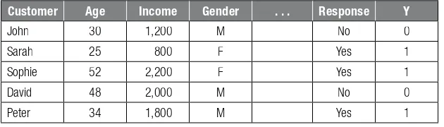
Consider a classifi cation data set for response modeling as depicted in Table 3.2 .
When modeling the response using linear regression, one gets:
= β + β + β + β
Y 0 1Age 2Income 3Gender
When estimating this using OLS, two key problems arise:
1. The errors/target are not normally distributed but follow a Bernoulli distribution.
2. There is no guarantee that the target is between 0 and 1, which would be handy because it can then be interpreted as a prob-ability.
Consider now the following bounding function:
= + −
f z
e z
( ) 1
1
which can be seen in Figure 3.2 .
For every possible value of z, the outcome is always between 0 and 1. Hence, by combining the linear regression with the bounding function, we get the following logistic regression model:
P response yes age income gender e
( | , , ) 1
1 (0 1age 2income 3gender)
= =
+ − β +β +β +β
The outcome of the above model is always bounded between 0 and 1, no matter what values of age, income, and gender are being used, and can as such be interpreted as a probability.
Table 3.2 Example Classifi cation Data Set
Customer Age Income Gender . . . Response Y
John 30 1,200 M No 0
Sarah 25 800 F Yes 1
Sophie 52 2,200 F Yes 1
David 48 2,000 M No 0
The general formulation of the logistic regression model then
Reformulating in terms of the odds, the model becomes:
P Y X X
or, in terms of log odds (logit),
= …