ISSN 1023-1935, Russian Journal of Electrochemistry, 2007, Vol. 43, No. 3, pp. 307–327. © Pleiades Publishing, Ltd., 2007.
Original Russian Text © N.D. Pismenskaya, V.V. Nikonenko, E.I. Belova, G.Yu. Lopatkova, Ph. Sistat, G. Pourcelly, K. Larshe, 2007, published in Elektrokhimiya, 2007, Vol. 43, No. 3, pp. 325–345.
1. INTRODUCTION
With an electric current flowing through an ion-exchange membrane, due to the difference between transport numbers for ionic components in the mem-brane and solution, there arises a concentration gradient of electrolyte in boundary layers of solution. In turn, this concentration gradient is the reason for the poten-tial near the membrane surface shifting away from its equilibrium value [1]. A similar phenomenon takes place in electrode systems as well [2]. This shift of potential is usually denoted by the term kontsentra-tsionnaya polyaritsatsiya (concentration polarization) in the Russian language literature [2] and overpotential or overvoltage in English [3, 4]. In the last case, the concentration polarization is understood to mean the current-induced formation of concentration gradients [5] (in a narrow meaning of the term) or the entire
com-plex of phenomena caused by the flowing of a current, including the formation of concentration gradients and secondary convective flows and other effects [6] (in a broad meaning of the term). According to notions of classic electrochemistry, the formation of concentration gradients near the membrane (electrode)/solution inter-face leads to a restriction that is imposed on the current density (i) by the so-called limiting current density (ilim). Once a zero concentration of electrolyte is
reached near a surface, i tends to limiting value ilim,
whereas a potential drop tends to infinity [2]. In real membrane and electrode systems, however, the density of a limiting current may be exceeded by several times at the expense of the emergence, near the surface of a membrane (electrode), of a complex of effects that are caused by concerted action of the flowing current and concentration variations in the system. These effects may be united by the term “coupled effects of concen-tration polarization” (CECP). Understanding these
Coupled Convection of Solution near the Surface
of Ion-Exchange Membranes in Intensive Current Regimes
N. D. Pismenskaya
a,z, V. V. Nikonenko
a, E. I. Belova
a, G. Yu. Lopatkova
a,
Ph. Sistat
b, G. Pourcelly
b, and K. Larshe
ca Kuban State University, ul. Stavropol’skaya 149, Krasnodar, 350040 Russia b Institut Europeen des Membranes, Montpellier, France
c Université Paris XII, Avenue du Général de Gaulle, Creteil, 94010 France Received May 16, 2006
Abstract—Mechanisms responsible for the overlimiting ion transfer in membranes systems are discussed. The overlimiting transfer is shown to be due largely to the action of four effects coupled with the concentration polarization of the system. Two of these are connected with the water dissociation near the membrane/solution interface: the emergence of additional charge carriers (ions H+ or OH–) in the depleted solution layer and the exaltation of transfer of salt counterions. The latter effect is connected with the perturbation of electric field caused by the water dissociation products. The other two effects are two versions of coupled convection, which leads to partial destruction of the depleted diffusion layer. These include gravitational convection and electro-convection. The former is caused by the emergence of the solution’s density gradient. The latter develops via a mechanism of electroosmotic slip. In this work, methods of voltammetry and chronopotentiometry and pH measurements are used to study the transfer of ions through homogeneous membranes Nafion-117 and AMX as a function of the concentration of sodium chloride solutions in the underlimiting and overlimiting current regimes. In a 0.1 M NaCl solution, gravitational convection makes a considerable contribution to the transfer of salt ions near the membrane surface in intensive current regimes. The influence of this effect on the electro-chemical behavior of membrane systems weakens with the solution dilution and with increasing relative trans-fer of the H+ and OH– ions that are generated at the membrane/solution interface. In conditions where gravita-tional convection is suppressed and the water dissociation near the membrane/solution interface is not great, the major contribution to the overlimiting growth of current is made by electroconvection. Topics for discussion in the paper include the mutual influence of effects on one another, in particular, the effect the rate of generation of the H+ and OH– ions exerts on the gravitational convection and electroconvection and the reasons for the dif-ferent behavior of cation- and anion-exchange membranes in intensive current regimes.
DOI: 10.1134/S102319350703010X
Key words: electrodialysis, overlimiting mass transfer, coupled convection, water dissociation
308 PISMENSKAYA et al. effects, which are responsible for the overlimiting mass
transfer, opens additional possibilities for intensifying electrolysis, electrodialysis, and electrodeionization of liquid media and makes it possible to broaden areas of application of these methods. In addition, exploring the coupled convection, which enters CECP, is of interest for perfecting electrokinetic micropumps [7], processes of electrophoresis [8, 9], electrodeposition [10], layer-ing colloidal crystals onto the surface of electrodes [11], and so on.
Four effects that explain the phenomenon of the overlimiting mass transfer are under discussion in the literature at present. Two of these are connected with the water dissociation at the membrane/solution inter-face. The emergence of additional charge carriers, namely the H+ and OH– ions that are generated during
the water dissociation in membrane systems [12–15], for a long time was considered as the principal and, fre-quently enough, sole, reason for the overlimiting con-duction [16]. At the same time, generation of the H+ and
OH– ions gives rise to another, less obvious, mechanism
of the overlimiting transfer. This is the effect of exalta-tion of a limiting current [2], which was explored as applied to electromembrane systems (EMS) for the first time by Yu.I. Kharkats [17]. The emergence of the H+
and OH– ions in the vicinity of the surface of a
mem-brane perturbs electric field and is capable of increasing (exalting) transfer of counterions of a salt. Consider, for example, the OH– ions, which are charged negatively.
When generated at the interface between a depleted dif-fusion layer and the surface of a cation-exchange mem-brane, these pull salt cations out of the solution depth towards the interface. With the effect of exaltation taken into account, the density of the flux of salt coun-terions (j1) is described by the equation [17]
(1)
where D1 and Ò0 are the diffusion coefficient for salt
counterions and concentration (for simplicity, 1 : 1) of electrolyte in the solution depth, δ is the thickness of a depleted diffusion layer (DDL), Dw and jw are the
sion coefficient and the density of a flux inside a diffu-sion layer of the water dissociation products that are generated near the surface of a membrane (in the case of a cation-exchange membrane, these are the OH–
ions). As follows from the Kharkats equation, i.e. equa-tion (1), the increment of the flux of salt counterions in excess of the limiting value j1 lim = 2Dic0/δ is
propor-tional to the flux of generated OH– (H+) ions, with a
proportionality coefficient being equal to D1/Dw.
The increase in the flux of salt counterions at the expense of the effect of exaltation in EMS is relatively not great. For example, it amounts to about 0.2 j1 lim in the case where the flux of the OH– ions reaches values
that are equal to j1 lim. In practice, the increment of salt
counterions is considerably greater [18–20] and, conse-quently, it cannot be explained by the effect of
exalta-j1
tion only. Other coupled effects must make a substan-tial contribution to the overlimiting transfer of salt counterions as well. Specifically, we speak here of two types of coupled convection, which provides for addi-tional, as compared with forced convection, agitation of solution. This particular agitation is caused by local vortexes that result from the action of bulk forces which are engendered by the flowing of an electric current. The first type of the coupled convection is a gravita-tional convection. It emerges owing to nonequilibrium distribution of density of solution, which is the reason for the emergence of a volume buoyancy force [21–23]. The second type is an electroconvection. It emerges as a result of the action of electric field on a space electric charge in the depleted solution adjacent to the mem-brane [6, 24–28].
The emergence of a bulk force in the case of gravi-tational convection is caused by gradients of concentra-tion and/or temperature [21–23]. This phenomenon is more probable in relatively concentrated solutions, for there take place in such solutions a stronger solution heating and a larger gradient of concentrations [22, 23], which are caused by a larger value of limiting density of an electric current, which is proportional, to a first approximation, to the solution concentration. In the case of a vertical solution/electrode (membrane) inter-face and the horizontal solution density gradient, the gravitational convection generally emerges in a thresh-oldless regime, i.e. it emerges always and gradually increases with the current (potential) [21]. The inter-face may be horizontal and the density of solution con-fined in between two parallel horizontal planes may alter along the perpendicular coordinate. Two cases are possible in such a situation. The lighter layer of solu-tion (depleted diffusion layer) may be posisolu-tioned under the membrane and the heavier layer of solution (enriched diffusion layer), above the membrane. In that case no convection emerges near the membrane. The lighter layer of solution may be positioned above the membrane. Then, a certain threshold takes place in the development of gravitational convection. The threshold in question is defined by the value of the Rayleigh num-ber [21–23]:
(2)
Here, Gr = is the Grashof number; Sc = ν/D is
a Schmidt number; ∆ρ is the change in the solution den-sity ρ, which occurs between the upper and lower por-tions of a layer of thickness X, in which the change in the solution density occurs; g is the gravitational accel-eration; ν is the solution viscosity; and D is the diffu-sion coefficient of electrolyte. A system is stable (i.e. no convection arises) if Ra < Racr = 1708. In such a case, the characteristic time that is required for the diffusion dissipation of the density fluctuation in a small volume
COUPLED CONVECTION OF SOLUTION NEAR THE SURFACE 309 of solution is shorter than the characteristic time
required for this volume to float up. At Ra > Racr, the volume with a negative density gradient floats up with acceleration, because the density inside a volume that is floating up increases slower than in the solution sur-rounding it. The amplitude of a small perturbation in this case increases with time, and the solution that is confined in between two planes achieves a certain state. This state is characterized by a periodic cellular vortex structure, where the liquid in two neighboring cells (Bénard convection cells) rotates in the opposite direc-tions [22, 23, 29]. Heat and mass transfer theory main-tains that gravitational convection in an “empty” (con-taining no spacer) rectangular channel is not suppressed by forced convection, provided Ri = Gr/Re2 > 1. Here, Ri
is the Richardson number and Re = VX/ν is the Rey-nolds number, where V is the average linear velocity of forced flow of solution [30, 31].
Research into the hydrodynamic instability due to gravitational convection in electrode systems was reviewed by V.M. Volgin and D.A. Davydov [23]. Results of mathematical modeling of this phenomenon in EMS were reported in [9, 19, 32, 33], for example. Gravitational convection plays a role in boosting the mass transfer and reducing the DDL thickness in inten-sive current regimes. This role was estimated experi-mentally using voltammetry and measuring partial transport numbers for ions [19, 20]. Its influence on the concentration polarization of EMS was probed with the aid of the chronopotentiometry [34] and laser interfer-ometry [5, 35] methods. Laser interferinterfer-ometry [5, 35] and microphotography with background laser illumina-tion were employed for observing convective moillumina-tion of liquid visually. In parallel, the structure of the Bénard convection cells was examined by the chronopotenti-ometry method [36, 37] with use made of a Fourier analysis of obtained curves. The sequence of events involved in the development of coupled convection near the surface of a homogeneous cation-exchange membrane was described in [38]. Using the Fourier and wavelet analyses, the authors of [38] showed that the frequency of revolutions of vortexes in a stationary state of EMS is equal to 0.1–0.4 Hz. This result con-forms to the data reported in [37], where it was estab-lished that the potential oscillations in chronopotentio-grams correlate with the life cycle of vortexes near the electrode/solution interface. The authors of [37] also demonstrated that the coupled convection may manifest itself at Ra < Racr = 1708 and explained this
phenome-non by the action of electrostatic forces, i.e. electrocon-vection.
According to modern theoretical notions, which were reviewed in [6, 25–28], the major mechanism governing the development of electroconvection in membrane systems is electroosmotic slip of second kind or, in terms of the authors of [24], who were the first to look into this phenomenon, “electroosmosis II.” Electroosmosis of second kind arises in membrane
sys-tems due to an electric field interacting with a space charge induced by this electric field. The space charge in question appears in DDL near the interface. As its extension increases in more dilute solutions [25, 39, 40], the electroconvection contribution to overlimiting mass transfer would presumably increase with decreas-ing salt concentration.
The space charge extension and density and the strength of the applied electric field are not the only fac-tors affecting the electroconvection intensity. The latter is also likely to depend on the Stokes radius of ions that make up the space-charge region. Indeed, the larger the Stokes radius of ions, the more efficient should be the involvement of the liquid into convective motion. The authors of [41] were probably the first to notice this cir-cumstance. Having compared current–voltage curves (CVC) recorded for a CMX membrane in various elec-trolytic solutions, they discovered that the plateau in CVC shrinks with increasing the Stokes radius of coun-terions. The shorter the plateau, the lower the voltage at which intensive coupled convection arose. They also observed that the EMS resistance decreased in overlim-iting regimes. The plateau length was maximum in a hydrochloric acid solution, for the H+ ions are
trans-ferred in solution via a relay mechanism, rather than a hydrodynamic mechanism [2]. Electroosmosis of sec-ond kind near granules of an ion-exchange resin, which were deployed in between two polarizing electrodes in a dilute solution, was confirmed experimentally in [25, 42].
The aim of this work is to experimentally investigate how the coupled convection influences electrochemical behavior of ion-exchange membranes and expose fac-tors that define its type and intensity in EMS. To do this, we will consider CVC and chronopotentiometric char-acteristics of homogeneous membranes under condi-tions favorable and not favorable for the development of coupled convection. We are also going to compare characteristics of cation- and anion-exchange mem-branes that have similar surface morphology but differ-ent capability to generate the H+ and OH– ions.
2. EXPERIMENTAL
2.1. Materials
310 PISMENSKAYA et al.
membrane Nafion-117 [45] relative to the water disso-ciation reaction is low [14]. The generation rate of the H+ and éç– ions on Nafion-117 is low, indeed. It is
substantially lower than that on AMX. The surface of both membranes is practically homogeneous and smooth (Fig. 1). The linear dimensions of small irregu-larities on it (protuberances, pits, bacteria, dirt
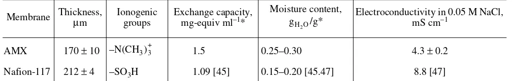
parti-cles, etc.) are 1–3 µm. The dimensions of microirregu-larities on the surface of membranes and in their bulk are connected with the technique used for manufactur-ing membranes. In the case of an AMX manufactured by a paste method [46], they lie in the limits from 100 to 300 nm. In the case of Nafion-117 produced by a method of polymerization [45], they do not exceed 30 nm. Basic characteristics of both membranes appear in Table 1. Values of the exchange capacity and mois-ture content were borrowed from [43, 45, 47].
The experiments were run at a temperature of (25 ± 1)°ë in 0.005, 0.02, 0.05, or 0.1 M solutions of NaCl, which were prepared from the reactant of analytical grade and distilled water with a resistance of no smaller than 0.5 Mohm and pH 5.5–6.2. Prior to experiment, membranes were equilibrated with a solution of a spec-ified concentration. In accord with recommendations of the firm-manufacturer, membranes Nafion-117 had first been subjected to a boiling procedure in distilled water for the duration of half an hour.
2.2. Investigation of the Surface of Membranes When obtaining micrographs of the surface and cross-section of membranes under study, we used a scanning electron microscope LEO (Leica, Cam-bridge), type S260. Prior to taking micrographs, mem-branes 24 h were kept in an exsiccator with a moisture absorber. The procedure used for preparing specimens was described in more detail in [34, 48].
2.3. Investigation of the Electrochemical Behavior of Membrane Systems
2.3.1. Experimental setup. The current–voltage curves, the chronopotentiograms, and the dependences of pH of near-membrane layers on the potential drop were obtained in a four-chamber cell of the flow-through type (Fig. 2a) that was described in [48]. The flow-through chambers of the flow-through cell are formed by membranes 1 as well as by plastic (Plexi-glas) frames 2 and rubber gaskets 3 and 4 with square holes of area S = 2 time 2 cm25. The thickness of the
Plexiglas frames had been fixed and equaled 4 or 5 mm. The distance between membranes can be varied by varying the thickness of the rubber gaskets 3 and 4. The chambers that are abutting the membrane under inves-3 µm
(‡)
3 µm (b)
Fig. 1. Photographs of surfaces of ion-exchange membranes (a) AMX and (b) Nafion-117.
Table 1. Principal characteristics of membranes under investigation
Membrane Thickness, µ m
Ionogenic groups
Exchange capacity, mg-equiv ml–1*
Moisture content,
/g* Electroconductivity in 0.05 M NaCl, mS cm–1
AMX 170 ± 10 –N(CH3 1.5 0.25–0.30 4.3 ± 0.2
Nafion-117 212 ± 4 –SO3H 1.09 [45] 0.15–0.20 [45.47] 8.8 [47]
* For swollen membrane in the Cl– form (AMX) of the Na+ form (Nafion-117). gH
2O
(‡)
1
2
3
4
5
6 8 7
9
10 11 A*
C A
22
5
18
17
21
23 19
20
15
12
14
13
25
8
24
16
9
Solution
Waste
Cell
pH
Autolab
pH
tigation A* on the side facing a flat platinum cathode 6 are separated by cation-exchange C and on the side of a flat platinum anode 7 by anion-exchange A mem-branes CMX and AMX, respectively. To take solution from near-surface layers of solution in order to monitor its pH, tips of two plastic capillaries 8 with an external diameter of about 0.8 mm are brought to the center of either side of the membrane under investigation. The end faces of the capillaries are situated in the immediate vicinity of the membrane at an angle of 45° to its sur-face. Two silver wires 9 with a diameter of 0.25 mm, which are covered with polyterefluoroethylene 0.024 mm thick squeezed in between rubber gaskets 3 and 4 from both sides of the membrane under investiga-tion. The end faces of these silver wires are fixed in the vicinity of capillaries 8 at a distance of approximately 0.8 mm from every side of the membrane under inves-tigation. They are covered with AgCl by means of polarization in the role of an anode in a 0.1 M solution of HCl for the duration of one hour at a current of 0.1 mA and serve for measuring the potential drop. The supply and removal of the feeding solution in each chamber is realized through connecting tubes 10 that are inserted into plastic frames. The devices for the solution insertion into a chamber and its removal out of it are performed in plastic frames in the form of comb 11 in order to provide for a laminar uniform flow of solution between membranes. The latter is necessary for alleviation of a mathematical description of transfer of ions in the cell, in particular, for calculation of the limiting current density and the diffusion layer thick-ness (Section 2.3.2.).
Figure 2b shows a schematic depiction of the exper-imental setup. The flow of liquid between membranes is ensured by the difference between hydrostatic pres-sures between the tube that removes solution out of cell 12 and intermediate reservoir 18 with the feeding solu-tion. Reservoir 18 with the aid of pump 17 is replen-ished by solution from reservoir 23 containing a siderably larger volume of the feeding solution. A con-stant level of solution in reservoir 18 is ensured by the hole 22, which is connected by means of a bendable hose with reservoir 23. In order to maintain a constant
hydrostatic pressure in the course of experiment, the exit tubes of cell 12 are fixed in the lid of auxiliary res-ervoir 24. Values of the flow velocity are regulated by valves 19, which are positioned on bendable tubes before the entrance into chambers of the cell.
Upon leaving capillaries 8, solution enters flow-through cells 13, into which combined glass and silver chloride electrodes WTW SenTix 97T 14 are placed. These electrodes are connected with the pH meters (pH-320 WTW) 15, which allow us to measure pH in flow-through cells 13. The rate of collecting solution for measuring pH in flow-through cells 13 is regulated by valves 25 that are deployed on short (8 cm) tubes, which connect capillaries 8 and flow-through cells 13. In order to ensure a specified hydrodynamic regime in chambers of cell 12, this rate must not exceed 5% of the rate of supply of solution into chambers of cell 12 that are abutting the membrane under investigation. When obtaining galvanodynamic CVC the time of “lag” of registered values of pH relative to the current values of the current tlag is defined by the volume of the
connect-ing tube W and the bulk velocity of solution flow w out of flow-through cells 13 (t
lag = W/w).
By rotating cell 12 it was possible to preset any angle between the membrane under investigation and the direction of the gravitational field of Earth. In this particular work we present results of experiments in which the membrane under investigation was situated in vertical or horizontal positions at an average velocity of the flow of solution. In the cases where the mem-brane under investigation is situated in a horizontal position, the current is directed in such a manner that the lighter depleted diffusion layer is situated below the membrane under investigation and the gravitational convection in the immediate vicinity of the membrane under investigation is absent (Section 1). If a cell is in a vertical position, solution is supplied into it from below upward.
In order to register potentials and specify currents, we used electrochemical complex 16 Autolab (Eco Chemie B.V., The Netherlands). The complex in ques-tion was equipped with a potentiostat PGSTAT 100 (Institut Europeen des Membranes, Montpellier, France) or a programmable power source Programma-ble Current Source 220, Keithley, and a high-resistance voltmeter Multimeter-3478A, Hewlett Packard (Uni-versity Paris XII, France) or potentiostat PI-50.1.1, and voltmeter V7-65/5 (Kuban State University, Russia). The specially designed software allowed us to realize digital recording of the measured potential drop with a minimum interval between signals equal to 0.01 s (Autolab) or 0.1 s (Multimeter-3478A) or 0.2 s (V7-65/5).
2.3.2. The treatment of experimental data: the limiting current density and the diffusion layer thickness. As it was established previously in [33], in the case of low currents, the mass transfer in the desali-nation channel of the cell under investigation is well Fig. 2. Schematics of (a) experimental cell and (b)
experi-mental setup for recording CVC and chronopotentiograms and measuring solution pH near the surface of the mem-brane under investigation: (1) membranes, (2) plastic frames, (3, 4) rubber gaskets, (5) square holes, (6) cathode, (7) anode, (8) plastic capillaries, (9) silver–silver chloride electrodes, (10) holes, (11) special comb, (12) experimental
described by a convective–diffusion model [40], pro-vided the desalination channel is formed by smooth homogeneous membranes. The model assumes a sta-tionary laminar forced convection of solution with a parabolic profile of velocity. To satisfy these conditions we used devices for supply and removal of solution 10 and 11 that were described in the foregoing (Fig. 2a). According to this model [40, 49], the limiting current density in a cell that is formed by smooth homogeneous ion-exchange membranes with a small value of desali-nation length Y = LD/Vh2 (on the order of 10–4, as is the
case in this work) is well described by the Leveck equa-tion
(3)
where Ò0 is the concentration of electrolyte at the
entrance to the desalination channel, L is the length of the active surface of the membrane under investigation, h is the intermembrane distance, V is the linear velocity of the flow of solution, T1 is the effective transport
num-ber of the salt counterion in the membrane, t1 is the
electromigration number of the salt counterion in the solution, and F is Faraday’s constant. The superscript “0” in the designation for the current density implies that we mean by it a quantity that would have taken place should there have been no coupled convec-tion.
Note that equation (3) has an approximate character. A more correct equation has a two-member right-hand part [40]. However, for simplicity we will use here the one-member equation (3) while keeping it in mind that the coefficient of proportionality in the right-hand part of (3) insignificantly varies with Y. Specifically, at Y = 10–4, this coefficient is equal to 1.47, as it is written in
equation (3); at Y = 10–2, however, its value is close to
1.43.
Another observation: the Poiseuille distribution of velocity may be violated if coupled convection of solu-tion arises in the system under investigasolu-tion. In that case one may expect that the experimental value of the limiting current density could be greater than the quan-tity calculated with the aid of the convective–diffusion model. Note that the experimental value of the limiting current density is determined approximately from the
ilim 0
1.47 FDc
0 h T( 1–t1) --- h
2 V LD
---⎝ ⎠ ⎛ ⎞1/3,
=
ilim 0
point of intersection of tangents drawn to the initial seg-ment at i = 0 and to the segment of slanted “plateau” in CVC.
The average value of the thickness of the depleted diffusion layer δ may be calculated after finding the limiting current density with the aid of equation (3) from the know equation
(4)
In the small-length electrodialysis channel under consideration we can presume that the concentration of electrolyte in the solution depth is identical to the con-centration c0 at the entrance into the cell. Equation (4)
is valid in the case where generation of the ç+ and éç–
ions at the membrane/solution interface is absent. Oth-erwise one should make use of the known Kharkats equation [17], i.e. equation (1), which takes into account the effect of exaltation of the current of salt counterions by the water dissociation products.
For calculations, the results of which are presented below, in all cases we used the following parameters: D = 1.61 × 10⁻⁵ cm2 s–1, = =0.998, t
Na = 0.396,
and tCl = 0.604 [50], where the superscript “C” refers to
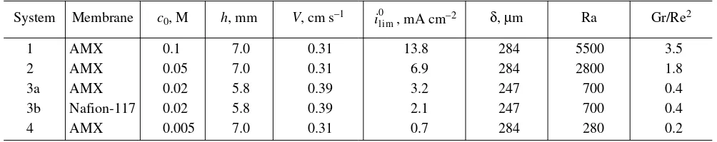
a cation-exchange membrane and the superscript “A” refers to an anion-exchange membrane. Other charac-teristics of the EMS under investigation are presented in Table 2 together with average values of the diffusion layer thickness. These values were calculated with the aid of equation (4) for the case where there takes place solely the forced convection.
The ratio between the salt concentration near the membrane surface and the salt concentration in the bulk solution in underlimiting current regimes is defined by the ratio [40, 49], see equation (A5) in Appendix. In the overlimiting current regimes, however, the ratio i/ilim defines the extension of the space-charge region
[39, 40]. Bearing this in mind, we deem it possible to state that the magnitude of the i/ilim ratio characterizes the degree of development of the concentration polar-ization. It is suitable to perform normalization of cur-rent density to quantity . The latter is easy to calcu-late with the aid of equation (3). Such a normalization allows us to compare the behavior of different
mem-ilim
0 FDc0
δ(T1–t1)
---. =
TNa C
TCl A
ilim0
ilim0 Table 2. Principal characteristics of electromembrane systems under investigation
System Membrane c0, M h, mm V, cm s–1
, mA cm–2 δ, µm Ra Gr/Re2
1 AMX 0.1 7.0 0.31 13.8 284 5500 3.5
2 AMX 0.05 7.0 0.31 6.9 284 2800 1.8
3a AMX 0.02 5.8 0.39 3.2 247 700 0.4
3b Nafion-117 0.02 5.8 0.39 2.1 247 700 0.4
4 AMX 0.005 7.0 0.31 0.7 284 280 0.2
brane systems at similar conditions of the development of coupled effects. It also makes it possible for us to estimate the influence of one effect or another on their electrochemical behavior.
The treatment of experimental data (continued): the potential drop. In the experimental cell we described in the foregoing, the total potential drop between two measuring electrodes (∆ϕtot) consists of the sum of
sev-eral potential drops as follows:
(5)
The first two addends in the sum are the potential drops that occur in the depleted (designated with super-script “I”) and enriched (supersuper-script “II”) diffusion lay-ers (DL). The third addend comprises the Donnan drops of potential on both membrane/solution interfaces (∆ϕDon). The last two addends refer to the ohmic drops
of potential on the membrane (∆ϕm) and in solution
lay-ers that are situated in between the measuring elec-trodes and the external boundaries of diffusion layers (∆ϕsol). The ∆ϕm and ∆ϕsol quantities are in essence ohmic drops of potential. The point here is that, in dilute solutions, the diffusion drop of potential in the membrane may be ignored [1] in view of the smallness of the concentration gradients. Moreover, in solution layers that are situated in between the measuring elec-trodes and the external boundaries of diffusion layers, concentration gradients are absent altogether.
When performing a comparison of the electrochem-ical behavior of different membrane systems with use made of voltammetry, it is convenient to use, instead of the total drop of potential ∆ϕtot, the quantity ∆ϕ', which
is defined by the equation
(6)
Here, Ref = (∂∆ϕtot/∂i)i=0 is the effective resistance of
the membrane system at low current densities, i.e. at i Ⰶ . This effective resistance includes the ohmic resistance of the space (membrane–solution) in between the measuring electrodes and the diffusion resistance of the depleted and enriched diffusion layers [3]. The value of this resistance is found from the slope of the initial segment of a CVC.
The ∆ϕ' quantity had been introduced probably by Maletzky et al. [51]. It was called a “reduced polariza-tion voltage” or a “reduced voltage of polarizapolariza-tion” (“corrected polarization voltage” in [51]). We will call it by the name “reduced drop of potential.” The ∆ϕ'
quantity shows the excess of a drop of potential in a sys-tem over the quantity that would have taken place upon retaining a linear growth of potential that is observed at i 0. The physical meaning of the ∆ϕ' quantity is close to overvoltage η [2–4]. Expressions for ∆ϕ' and η are derived in Appendix. Resorting to the reduced drop of potential ∆ϕ' allows us to exclude from consideration the initial ohmic resistance. The latter is dependent on
∆ϕtot ∆ϕDL
the separation between the measuring electrodes, the membrane thickness, and some other parameters. These parameters are frequently not that important for the behavior of a membrane but are difficult to take into account upon going from one membrane system to another.
To compare results obtained during chronopotenti-ometry of different membrane systems, the difference between potentials ∆ϕtot and ∆ϕOhm is used. The ohmic constituent ∆ϕOhm = iRohm is found as the potential drop
between measuring electrodes that is caused by switch-ing a current on under conditions where concentration gradients are absent. In practice, the value of ∆ϕOhm is
found from a chronopotentiogram by means of extrap-olation of ∆ϕtot at t 0. The ohmic constituent ∆ϕOhm
comprises the ohmic drops of potential in all layers of a system that consists of a membrane, two diffusion layers, and two layers of solution in between the mea-suring electrodes and external boundaries of the diffu-sion layers. The difference between the ohmic resis-tance Rohm and the effective resistance Ref of a system is
defined by equation (A8). The difference in question consists of that the effective resistance Ref, apart from
the ohmic resistance Rohm, includes diffusion resis-tance, which arises upon establishing a concentration profile in EMS [3, 4].
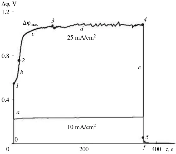
The treatment of experimental data (continued): chronopotentiometry. At current densities below or equal to , chronopotentiograms for the diffusion-controlled EMS with a smooth mass exchange surface have the shape presented in Fig. 3 [34, 46, 48]. The ini-tial portion of the curve contains three segments. Seg-ment ‡, confined by point 1 in Fig. 3, is practically ver-tical. Its height is defined by the value of the total ohmic resistance of the membrane and two layers of solution that are confined in between the measuring electrodes and the membrane at = = c0. The slope of this
segment at t 0 depends on the capacitance of the electrical double layer (EDL) at the membrane/solution interface [52]. Segment b corresponds to a slow build-ing up of the potential until inflection 2. This magnifi-cation of the potential is caused by a decrease of con-centration in the solution layer near the membrane that undergoes desalination. At point 2 the potential rises at a maximum rate. Thereafter the potential growth rate diminishes and the potential drop ∆ϕ reaches a certain steady-state value or a quasi-steady-state value (seg-ment d). In the quasi-steady state, the potential drop ∆ϕ slowly alters or periodicaly oscillates. The fact that the growth of ∆ϕ slows down testifies to the amplification of coupled effects, in the first place, of the coupled con-vection. These effects reduce the degree of concentra-tion polarizaconcentra-tion of the system. Note that in segment d the potential drop ∆ϕ is equal to the potential drop that is observed in galvanostatic or galvanodynamic CVC that are recorded at a low rate of the current scan (~0.01 mA s–1). The shape of the time dependences of
ilim0
∆ϕ and the character of oscillation of this potential drop in segments c and d yield information concerning the type and the scenario of the development of coupled effects of concentration polarization. The last segment, denoted as f, is obtained after switching the current off. It describes the process of diffusion relaxation of the system.
The simplest mathematical model for semiinfinite diffusion toward a flat mass exchange surface is the Sand model [52]. It takes no account of the coupled effects of concentration polarization. The model has parameter τ that is called a transition time. This param-eter is defined by the following expression [46]:
. (7)
In the framework of this model, parameter τ corre-sponds to the time instant when the electrolyte concen-tration near the surface of a membrane turns zero and the potential drop tends to infinity. The concentration of counterions in the solution depth in the systems we are investigating is presumably none other than the con-centration c0 of a 1 : 1 electrolyte at the entrance into the
cell. As follows from equation (7), the magnitude of the product iτ1/2 is independent of the current density in the
overlimiting current regimes. This statement is true if the mass transfer in the electrochemical system is con-trolled by electrodiffusion not complicated by coupled effects of concentration polarization. From the view-point of some modern notions, the quantity τ may be defined as the time period required for the electrolyte
τ πD
4
---⎝ ⎠ ⎛ ⎞ ci
0 ziF Ti–ti
---⎝ ⎠ ⎛ ⎞21
i2 ---=
ci 0
concentration in the vicinity of the membrane/solution interface to drop to such values csⰆc0 at which
cou-pled effects start manifesting themselves. The action of these effects is manifested in the slowing-down of the magnification of the potential drop ∆ϕ. Consequently, the transition time may be approximately determined from the inflection point 2.
The potential difference between points 4 and 5 in Fig. 3 (segment e) is equal to the ohmic drop of poten-tial of a polarized membrane system. The potenpoten-tial dif-ference ∆ϕ4–5
– ∆ϕ1
corresponds to the change in the ohmic drop of potential in EMS that is caused by the development of concentration polarization. The major contribution to this quantity is made by the increment of the resistance of the depleted diffusion layer:
∆Rδ≈ (∆ϕ4–5 – ∆ϕ1)/I. (8)
3. RESULTS AND DISCUSSION
3.1. Effect of Concentration Polarization on the Gravitational Convection
As we have already mentioned in Introduction, a rather simplistic analysis demonstrates that the gravita-tional convection weakens with decreasing salt concen-tration in solution. The degree, to which the gravita-tional convection has developed, may be prognosti-cated with the aid of values of the Rayleigh number Ra and the Richardson criterion Ri = Gr/Re2. Calculations
of these quantities for conditions that were used in this work were performed with the aid of formula (2) for a temperature of 25°ë. The calculations were conducted ∆ϕmax
200 400
0 0.4 0.8
2
1 1.2
4 3
a b
c d
e
5 10 mA/cm2
25 mA/cm2
f ∆ϕ, V
t, s 0
under the assumption that characteristic distance X may be estimated as the total thickness of a diffusion layer
δtot. Here, the characteristic distance X is the size of the
region where the solution density gradient is other than zero. As to the total diffusion layer thickness δtot, it is
determined from the point where salt concentration differs by a mere 1% from the value of c0,
which is the salt concentration in the solution depth. In the cases of forced [49] and natural [53] convection of solution, the total diffusion layer thickness is ~1.7 times the Nernst layer thickness δ [40]. Then, δtot = 1.7 ×0.028 ≈ 0.05 (cm) for systems 1, 2, and 4 in Table 2 and δtot =1.7 × 0.025 ≈ 0.04 (cm) for systems 3a and 3b in the same table. When performing calcula-tions we assumed that the difference between densities of a 0.1 M NaCl solution (external boundary of a total depleted diffusion layer) and pure water (near the
inter-face, at i ≥ ) is equal to 0.004 g cm–3 and decreases c x δ
tot =
ilim 0
proportionally to concentration c0. The viscosity ν was
set equal to 0.009 cm2 s–1. The solution flow velocities,
which are required for calculating the Reynolds num-ber, appear in Table 2. The estimate was conducted without allowance for possible heating of solution near the interface.
As expected, values of the Rayleigh number and the Richardson criterion diminish with the solution dilution (Table 2). In the case of a 0.1 M NaCl solution (system 1 in Table 2), Ra >Racr and Gr/Re2Ⰷ 1. This
implies that the conditions that are required for the emergence of gravitational convection are created if the depleted diffusion layer is not situated under the mem-brane. In the 0.05 and 0.02 M NaCl solutions (systems 2 and 3 in Table 2), values of Ra and Ri are almost critical. This points to a weak contribution of gravitational convection. The contribution may be increased or decreased due to heat evolution or con-sumption near the membrane surface, which is ignored by calculations of the Rayleigh and Grashof numbers. The development of gravitational convection in a 0.005 M NaCl solution (system 4 in Table 2) is hardly probable.
The obtained experimental data (Figs. 4–6) corrob-orate the validity of the estimates we made and corre-late with the results reported in [19, 20]. In the case of a 0.1 M NaCl solution (system 1 in Table 2), the shape of the current–voltage curves (Figs. 4, 5) and the chro-nopotentiograms (Fig. 6) that were recorded at current densities in excess of substantially depends on the membrane’s position: vertical or horizontal. (In this case and in what follows, for a membrane in the hori-zontal position, the electric field is oriented so that the lighter depleted diffusion layer is situated under the membrane under investigation, which practically rules out the emergence of gravitational convection in the vicinity of this membrane.)
Let us compare curves 1
G and 1V in Fig. 5a, which
were obtained for AMX deployed in, respectively, hor-izontal and vertical positions in a 0.1 M NaCl solution. The slope of the portion of the “plateau” in the CVC for the AMX membrane positioned horizontally is very small and the length of the plateau is large enough, which testifies to considerable diffusion limitations that hamper the mass transfer in this portion. The value of the limiting current density ilim that was found from the
intersection of tangents as described in Subsection 2.3.2 is very close to the value of that was calcu-lated with the aid of equation (3). The evaluations made using formula (A9) (Appendix) suggest that the salt concentration cs near the membrane surface decreases
at i = by four orders of magnitude as compared with the concentration in the depth of solution (the cal-culation was made on the basis of the known potential drop at this current density). Upon going from the hor-izontal position to the vertical position, which is
favor-ilim0
ilim0
ilim 0
∆ϕ', V
1 2 3 4
i/i0lim 0
1 2
1pH
2V
2pH 4V
1V
–2 0
–1 ∆pH
4pH
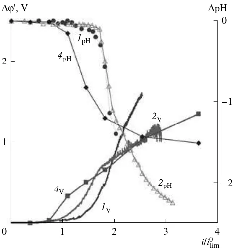
Fig. 4. Dependences of the corrected potential drop of con-centration polarization and variations in the pH value of a near-membrane layer of depleted solution on the current
density normalized to the limiting current , which was calculated with the aid of equation (3) for the AMX mem-brane at h = 7.0 mm and V = 0.32 cm s–1. The calculations are performed for the following different values of the NaCl solutions: (1
G, 1V, 1pH) 0.1, (2G, 2V, 2pH) 0.5, and (4G, 4V,
4
pH) 0.05 M. Points represent data obtained in galvanostatic regime and curves refer to data obtained in galvanodynamic regime with the current scanned at a rate of 0.01 mA s–1. Subscripts “h,” “v,” and “pH” denote, respectively, horizon-tal and vertical positions of the membrane under investiga-tion and the soluinvestiga-tion pH. Numbers identifying the curves correspond to numbers of systems in Table 2.
able for the development of gravitational convection (Fig. 5a, curve 1
V), similar values of the salt
concentra-tion cs occur solely at i≈1.55 . The value of the
lim-iting current density that is determined from the inter-section of tangents is approximately 1.5 times the value of . A subsequent build-up of the preset current leads to the appearance of a plateau in curve 1
V in
Fig. 5a. However, the slope of this plateau is smaller than that for the membrane in the horizontal position. These data point to the removal of a part of the diffusion limitations in the case of the membrane positioned ver-tically, due to the development of gravitational convec-tion near its surface.
A twofold decrease in the concentration of the feed-ing solution (system 2 in Table 2) leads to a substantial shrinkage of differences in the behavior of AMX deployed in a horizontal position (Fig. 5a, curve 2G) and in a vertical position (Fig. 5a, curve 2
V). For the
same membrane in a 0.005 M NaCl solution (system 4 in Table 2), these differences are practically absent (Fig. 5a; curves 4G, 4V). The absence of these differ-ences testifies to a negligibly small influence the gravi-tational convection exerts on the mass transfer in this particular system.
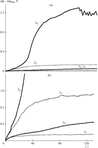
Note that the gravitational convection in the AMX−0.1 M NaCl system starts manifesting itself as early as at current densities below the limiting current density. However, the influence exerted by it is not great. At i = 10 mA cm–2 (i/ = 0.7), for example, the
difference ∆ϕtot – ∆ϕOhmfor the AMX membrane in the horizontal and vertical positions does not exceed 0.025 V in the quasi-steady state (Fig. 6; curves 1
G, 1V).
At higher current densities, this difference is greater. The difference is maximum at such current densities that are limiting or overlimiting in the horizontal posi-tion but are still underlimiting in the vertical posiposi-tion. The case where i = 20 mA cm–2 is a good example. A
calculation with (3) for this case yields i/ = 1.4. The clearly pronounced portion of the transition time (Fig. 6, curve 2
G) testifies to the reaching of the limiting
state by the membrane positioned horizontally. At the same time, for the vertical position, the portion of the transition time is absent and the steady-state drop of potential reaches a mere ~0.100 V (Fig. 6, curve 2V).
As follows from Fig. 6b, within the first seven sec-onds after switching the current on, the chronopotentio-gram that was recorded at i = 20 mA cm–2 in the vertical
position of AMX repeats the run of the curve for the same membrane that was obtained for the horizontal position. This time period may be referred to the time period required for the development of gravitational convection after switching the current on. After the “splitting” of curves, the difference ∆ϕtot – ∆ϕOhm
sharply increases for the membrane in the horizontal position. Conversely, for the membrane in the vertical position, the growth of this difference sharply slows
ilim 0
ilim 0
ilim 0
ilim0
down, and low-frequency oscillations of potential appear in the chronopotentiogram. The period of these oscillations is equal to 7–8 s and their amplitude is low. Emulating the authors of [37], we deem it possible to assume that the period of oscillation of potential corre-sponds to the time period that elapses from the instant ∆ϕ', V
1 2 3
0 1 2
3bV
(b) 3‡V 3
3bG 3‡G
1 2
i/i0lim
0 1 2
2V (‡)
1V 3
1G 2G 4
4G, 4V
Fig. 5. Dependences of current density normalized to the
limiting current density on the corrected potential drop of concentration polarization for membranes (a, b) AMX and (b) Nafion-117. Curves in panel a are obtained at NaCl concentrations equal to (1G, 1V) 0.1, (2
G, 2V) 0.5, and (4G,
4V) 0.05 M and h = 7.0 mm, V = 0.32 cm s–1. Panel b: 0.02 M NaCl, h = 5.8 mm, V = 0.39 cm s–1. Numbers iden-tifying the curves correspond to numbers of systems in Table 2.
when two successively engendered vortexes arise in the vicinity of a measuring electrode, i.e. the oscillation period corresponds to the lifetime of a vortex. In the system that we have studied, this time period has the same order of magnitude as the time period that was found by the authors of [38] when analyzing flicker noise of a CVC of an electromembrane system. The amplitude of the potential oscillations is probably defined not only by the magnitude of the change that
occurs in the concentration of solution in the vicinity of the membrane surface but by the site of location of measuring electrodes as well.
Note the presence of oscillations of potential with a period of oscillations equal to 3–4 s in segment d of the chronopotentiogram that was obtained at a current den-sity of 20 mA cm–2 for the AMX membrane deployed
in the horizontal position (Fig. 6a, curve 2
G). The
oscil-lations are connected probably with electroconvection. ∆ϕ – ∆ϕohm, V
0 0.4 0.8
(‡)
2V 1.2
2G
1G, 1V
40 80 120
0 0.5 0.1
(b)
2V
0.15 2G
1G
1V
t, s
Fig. 6. (a) Chronopotentiograms for the AMX membrane in horizontal (subscript “h”) and vertical (subscript “v”) positions in a
0.1 M NaCl solution ( = 0.1 å, h = 7.0 mm, V = 0.32 cm s–1), obtained at the following current densities: (1
G, 1V) 10 and (2
G, 2V) 20 mA cm–2. Panel b: initial segments of the same chronopotentiograms in an enlarged scale.
It should be noted that values of transition times that were found from experiment on the basis of the maxi-mum of derivative d(∆ϕtot – ∆ϕOhm)/dt, which
corre-sponds to the inflection in a chronopotentiogram, for the AMX membrane that was placed in the horizontal position practically coincide with the value that were calculated with the aid of the Sand formula, i.e. formula (7). This situation holds for all concentrations of the NaCl solution studied in this work (Fig. 7). At the same time, for the AMX membrane placed in the vertical position in a 0.1 M NaCl solution at current densities in the region 1.3 < i/ < 2.9, experimental values of τ
exp
exceed values that are predicted by equation (7). As seen in Fig. 7, the difference between values of (iτ1/2)
exp
and (iτ1/2)
Sand shrinks with increasing current density
and with solution dilution. For example, for the AMX membrane at i/ = 2 for concentrations equal to 0.1 and 0.05 M, this difference amounts to 17 and 10%, respectively. In more dilute solutions (0.02, 0.005 M NaCl), the difference does not exceed 3%. The observed excess of experimental transition time τexp
over the transition time calculated with the Sand for-mula, τSand, may presumably serve as a measure
reflect-ing the contribution made by the gravitational convec-tion to the mass transfer process. Specifically, gravita-tional convection arises under conditions where the boundary concentration is not necessarily very low, i.e.
ilim0
ilim0
at times that are far shorter than the transition time. The more intensive the gravitational convection, the more efficient the supply of fresh solution toward the mem-brane surface and, consequently, the slower the process of desalination of solution near the interface and the larger the excess of the transition time over the calcu-lated value. It will be remembered that the Sand equa-tion had been derived under the assumpequa-tion that the sole mechanism of the supply of an electrolyte toward the surface of a solid body is electrodiffusion through a stagnant semi-infinite layer of solution [52].
3.2. Effect of Generation of the ç+
and éç–
Ions in a Membrane System on the Coupled Convection
The effect of generation of the ç+ and éç– ions in
a membrane system on the mass transfer is not unam-biguous. On one hand, as we mentioned in Introduc-tion, at the expense of the exaltation effect, this process may slightly raise the density of the current correspond-ing to the flow of salt counterions. On the other hand, these ions force the salt counterions out of the space-charge region. The forcing-out process hampers elec-troconvection via the mechanism of electroosmosis of second kind. This happens because the Stokes radius of salt counterions is much greater than the Stokes radius of the ç+ and éç– ions. Note that the Stokes radius of
the ç+ and éç– ions is close to zero as a consequence
of some specific features pertaining to the mechanism i/i0lim
1 2
0 40 80
1V
2V 120
2G
3‡G, V iτ1/2
1G
i/i0lim, V
2 6
0 10 12 14
3bG iτ1/2
4 3bV
Fig. 7. Dependences of product iτ1/2 on the current density normalized to the limiting current density . The dependences were obtained for an EMS whose numbers in Table 2 corresponds to the curves' numbers. Points refer to experimental data. Curves
rep-resent results of calculations with the aid of the Sand equation, i.e. equation (7). Vertical dashed line marks i = .
ilim0
of their transfer. Finally, of importance is the heat effect occurring during the generation of the ç+ and éç– ions
and in the course of their recombination.
3.2.1. Factors that define the rate of generation of the ç+
and OH–
ions. The rate of generation of the H+
and OH– ions may be judged upon on the basis of the
difference between values of pH of the feeding solution and the solution abutting the membrane (flowing out of capillaries 8 in Fig. 2). In Fig. 4 we show results of measurements of pH of a depleted boundary solution, obtained for a membrane placed in the vertical position, as a function of the value of the i/ ratio. As follows from an analysis of these data as well as from an anal-ysis of CVC (Figs. 4, 5), variations of pH in the vicinity of the surface of anion-exchange membrane AMX begin to be fixed at current densities icr (the current of
the commencement of generation of the H+ and OH–
ions) that are close to ilim. This observation holds for all
concentrations of sodium chloride studied in this work. The commencement of noticeable dissociation of water must correspond to the reaching of a threshold concen-tration of sodium chloride cs near the interface. The threshold concentration of sodium chloride is the con-centration at which the relative concon-centration of the generated H+ (OH–) ions rises to such an extent that the
transport numbers for the H+ and OH– ions in the
near-membrane region of solution turn commensurate with the transport numbers for the salt counterions. The threshold concentration is on the order of 10–5 M, if we
take into account that the mobility of the H+ and OH–
ions is about ten times the mobility of the salt counteri-ons and that the equilibrium concentraticounteri-ons of the prod-ucts are on the order of 10–7 M. In that case, the
trans-port numbers for the H+ and OH– ions in a solution
layer bordering the membrane must become suffi-ciently large (approximately 0.1) in order to ensure per-ceptible variations of pH. Estimates of the threshold value of the drop of the potential of concentration polarization (∆ ), at which water dissociation becomes tangible, may be made with the aid of equa-tion (A10), which is presented in Appendix. For a 0.1 M NaCl solution, equation (A10) gives ∆ = 0.406 V, whereas ∆ = 0.252 V for Ò0 = 0.005 M.
Experimental values that were determined for the AMX membrane placed in the vertical position amount to
0.380 ± 0.030 V (Fig. 4; curves 1V, 1pH) and 0.280 ± 0.020 V (Fig. 4; curves 4
V, 4pH). Following a further
increase in a voltage (current density), cs goes on
decreasing and the current of the H+ (OH–) ions
contin-ues increasing in accord with the following relationship [54]:
(9)
Expression (9) was derived in [54] with use made of theory of water dissociation in bipolar membranes [13–
ilim0
15] and the results of solutions of the Nernst–Planck– Poisson equations [39, 40]. Coefficients A
1 and β1 in (9)
are independent of the current density. However, these coefficients depend on the structure of the membrane surface, the diffusion layer thickness (β1), and the
cata-lytic activity of fixed groups relative to the water disso-ciation reaction and the solution concentration (A
1).
This catalytic activity is defined by the rate constant of the klim. It is increasing in the following series [12, 14]:
(10)
Indeed, no noticeable alkalization of the boundary solution on the side of the depleted diffusion layer was fixed near sulfuric acid membrane Nafion-117 that was situated in a 0.02 M NaCl solution (system 3b in Table 2). This observation is true for all the current den-sities studied in this work. On the other hand, as we have already discussed it in the foregoing, the acidifica-tion of soluacidifica-tion near the AMX membrane, which con-tains secondary and tertiary amino groups [44], may be very substantial. In the case of AMX, the pH vs. i/
dependences for systems 1 and 2 (Table 2), which have close values of icr, are practically identical (Fig. 4;
curves 1
pH, 2pH). This fact confirms the validity of
equa-tion (9) one more time. Specifically, as follows from this equation, the flux of the H+ (OH–) ions generated in
the overlimiting current regimes is proportional to the i/ilim ratio, provided catalytic activity with respect to the
water dissociation reaction is fixed and the surface mor-phology is identical.
3.2.2. Estimation of the effect the water dissocia-tion reacdissocia-tion exerts on heat effects. The water disso-ciation reaction is endothermic. Conversely, during the formation of water, heat evolves:
H+ + OH– H
2O + ∆H. (11)
Here, ∆H is the heat of chemical reaction, which equals –56.7 kJ mol–1 at 25°ë [50]. Consequently, in
elec-tromembrane systems with intensive water dissociation in the vicinity of the membrane/solution interface, one may expect that the gravitational convection is weaker. The weakening could be due to the consumption of a fraction of heat that was generated because of the Joule heating at the interface.
The amount of heat (as calculated per unit area of surface) that is consumed in the vicinity of the interface as a result of the occurrence of the water dissociation reaction may be estimated with the aid of the following formula:
(12)
The increment of the Joule heat, which is generated in the depleted diffusion layer adjacent to the membrane and which is caused by an increase in the resistance of the depleted diffusion layer that occurs at the expense
–N CH( 3)3+<–HSO3–<–NH2,= NH
klim, s–1 0 3 × 10⁻³ 10–1
ilim 0
of concentration polarization, may be estimated approximately as follows:
(13)
Values of the difference ∆ϕ4–5 – ∆ϕ1 in this equation
are determined from the chronopotentiograms given in Fig. 3. These values correspond to the change in the ohmic drop of potential that is caused by the develop-ment of concentration polarization in the electrobrane system. The ohmic drop of potential in the mem-brane and in the enriched diffusion layer hardly alters in the course of formation of concentration profiles. As a result, the magnitude of the difference ∆ϕ4–5
– ∆ϕ1
is indeed caused chiefly by the increase in the resistance of the depleted diffusion layer.
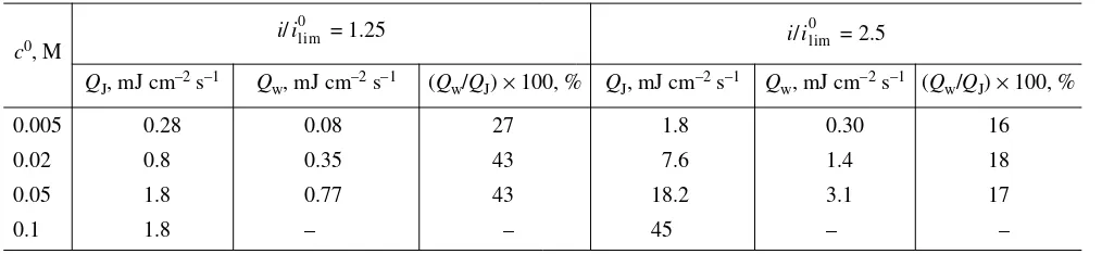
Figure 8 presents dependences of QJ on i/ , which
were obtained at different concentrations of the NaCl solution in an EMS with the AMX membrane placed in the vertical position. As seen in Fig. 8, at concentrations of NaCl equal to 0.02–0.1 M, the amount of the gener-ated Joule heat commences to discernibly rise at i/ > 1.5, when substantial changes of the potential drop in the depleted diffusion layer are reached. As expected, QJ is most significant in a 0.1 M NaCl
solu-tion and decreases with its dilusolu-tion. At a fixed value of i/ , the resultant Joule heating weakens not propor-tionally to the decrease in the solution concentration but more severely (Table 3). The reason for this phe-nomenon is the decrease in the potential drop ∆ϕ4–5
–
∆ϕ1
, which is caused by the decrease in the solution concentration.
In Table 3 we perform a comparison of values of QJ
and Qw that were computed with the aid of equations
(12) and (13), respectively. In the calculations we used values of the transport number TOH for the OH– ions
through the AMX membrane that were equal to 0.15 and 0.3 for i/ of 1.25 and 2.5, respectively. These values had been obtained in a special experiment using the procedure of maintaining the concentration and pH value of the feeding solution constant [20, 40] for the AMX–CMX system at h = 1.0 mm, L = 3 cm, V = 1.6 cm s–1, and Ò0 = 0.005 M (i
lim = 1.98 mA cm–2, δ = QJ = (∆ϕ4–5–∆ϕ1)i.
ilim 0
ilim0
ilim 0
ilim0
100 µm). Bearing in mind notions that were developed in [54], it was presumed that the value of TOH, which
was determined for the given value of the i/ ratio, would be the same as in the systems under investigation in this work. No calculation of Qw for the concentration Ò0 = 0.1 M was performed, for an intensive gravitational
convection in this system may lead to a noticeable devi-ation from equdevi-ation (9).
A comparison of values of QJ and Qw given in
Table 3 yields the following results. At i/ = 1.25 and sodium chloride concentrations equal to 0.005–0.05 M, the heat that is consumed at the expense of the water dis-sociation reaction may amount up to 40% of the Joule
heat. According to the estimates we made, with i/
raised to 2.5, the fraction of the absorbed heat dimin-ishes to 20%. Thus, the Joule heating becomes ever more substantial with increasing current density. This conclusion conforms to the experimental data to be
ilim0
ilim0
ilim 0
2 4 6
0 20
40 1
60
i/i0lim 2
3a
4 QJ, mJ cm–2 s–1
Fig. 8. Dependences of the Joule heat on the current density normalized to the limiting current density , obtained for systems 1, 2, 3a, and 4 (Table 2) with an AMX membrane placed in the vertical position in solutions containing (1) 0.1, (2) 0.5, (3a) 0.02, and (4) 0.005 M NaCl.
ilim0
Table 3. Evaluation of heat effects in a electromembrane system with the AMX membrane
c0, M
i/ = 1.25 i/ = 2.5
QJ, mJ cm–2 s–1 Qw, mJ cm–2 s–1 (Qw/QJ) × 100, % QJ, mJ cm–2 s–1 Qw, mJ cm–2 s–1 (Qw/QJ) × 100, %
0.005 0.28 0.08 27 1.8 0.30 16
0.02 0.8 0.35 43 7.6 1.4 18
0.05 1.8 0.77 43 18.2 3.1 17
0.1 1.8 – – 45 – –