Gunnar Stiesch · Frank Otto
with 242 figures
1 3
Simulating Combustion
Simulation of combustion and pollutant formation
Prof. Dr.-Ing. habil Günter P. Merker Universität Hannover
Institut Technische Verbrennung Welfengarten 1 A
30167 Hannover
Prof. Dr.-Ing. Christian Schwarz BMW-Group, EA 31
Hufelandstr. 8a 80788 München
isbn 10 3-540-25161-8 Berlin Heidelberg New York isbn 13 978-3-540-25161-3 Berlin Heidelberg New York
This work is subject to copyright. All rights are reserved, whether the whole or part of the material is concerned, specifi cally the rights of translation, reprinting, re-use of illustrations, recitation, broadcasting, reproduction on microfi lms or in any other way, and storage in data banks. Dupli-cation of this publiDupli-cation or parts thereof is permitted only under the provisions of the German Copyright Law of September 9, 1965, in its current version, and permission for use must always be obtained from Springer. Violations are liable to Prosecution under the German Copyright Law. Springer is a part of Springer Science+Business Media
springeronline.com
© Springer-Verlag Berlin Heidelberg 2006 Printed in Germany
The use of general descriptive names, registered names, etc. in this publication does not imply, even in the absence of a specifi c statement, that such names are exempt from the relevant protec-tive laws and regulations and free for general use.
Cover design: medionet AG, Berlin
Typesetting: Digital data supplied by editors
Printed on acid-free paper 68/3020/m-5 4 3 2 1 0
Dr.-Ing. habil Gunnar Stiesch
MTU Friedrichshafen GmbH, Abtl. TKV Maybachplatz 1
88045 Friedrichshafen
Dr. rer. nat. Frank Otto
DaimlerChrysler AG, Abtl. HPC G252 70546 Stuttgart
Library of Congress Control Number: 2005933399
Originally published as
Günter P. Merker/Christian Schwarz/Gunnar Stiesch/Frank Otto:
Verbrennungsmotoren. Simulation der Verbrennung und Schadstoffbildung
The numerical simulation of combustion processes in internal combustion engines, including also the formation of pollutants, has become increasingly important in the recent years, and today the simulation of those processes has already become an indispensable tool when de-veloping new combustion concepts. While pure thermodynamic models are well-established tools that are in use for the simulation of the transient behavior of complex systems for a long time, the phenomenological models have become more important in the recent years and have also been implemented in these simulation programs. In contrast to this, the three-dimensional simulation of in-cylinder combustion, i.e. the detailed, integrated and continuous simulation of the process chain injection, mixture formation, ignition, heat release due to combustion and formation of pollutants, has been significantly improved, but there is still a number of challenging problems to solve, regarding for example the exact description of sub-processes like the structure of turbulence during combustion as well as the appropriate choice of the numerical grid.
While chapter 2 includes a short introduction of functionality and operating modes of internal combustion engines, the basics of kinetic reactions are presented in chapter 3. In chapter 4 the physical and chemical processes taking place in the combustion chamber are described. Chap-ter 5 is about phenomenological multi-zone models, and in chapChap-ter 6 the formation of pollut-ants is described. In chapter 7 and chapter 8 simple thermodynamic models and more com-plex models for transient systems analyses are presented. Chapter 9 is about the three-dimensional simulation of combustion processes in engines.
We would like to thank Dr. B. Settmacher for reviewing and formatting the text, for preparing the layout, and for preparing the printable manuscript. Only due to her unremitting dedication and her excellent time management the preparation of this book has been possible in the given timeframe. Further on, we would also like to thank Mrs. C. Brauer for preparing all the figures and diagrams contained in this book. The BMW group and the DaimlerChrysler AG contributed to this book by releasing the figures they provided. Last but not least, we would like to thank the Springer-Verlag for the always excellent collaboration.
This book is largely a translation of the second German edition, which has been published in 2004 by the B.G. Teubner-Verlag, whereas the text has been updated if necessary. We would like to thank Mr. Aaron Kuchle for translating the text into English.
Hannover/München/Friedrichshafen/Stuttgart, July 2005 Günter P. Merker
Christian Schwarz
Gunnar Stiesch
Table of contents
Abbreviations and symbols
XII1 Introduction
11.1 Preface 1
1.2 Model-building 1
1.3 Simulation 2
2 Introduction into the functioning of internal combustion engines
52.1 Energy conversion 5
2.2 Reciprocating engines 6
2.2.1 The crankshaft drive 7
2.2.2 Gas and inertia forces 9
2.2.3 Procedure 11
2.3 Thermodynamics of the internal combustion engine 12
2.3.1 Foundations 12
2.3.2 Closed cycles 17
2.3.3 Open comparative processes 25
2.4 Characteristic qualities and characteristic values 28
2.5 Engine maps 31
2.5.1 Spark ignition engines 31
2.5.2 Diesel engines 33
2.6 Charging 35
2.6.1 Charging methods 35
2.6.2 Supercharging 37
2.6.3 Constant-pressure turbocharging 38
2.6.4 Pulse turbocharging 41
3 Foundations of reaction kinetics
443.1 Chemical equilibrium 44
3.2 Reaction kinetics 47
3.3 Partial equilibrium and quasi-steady-state 48
3.4 Fuels 50
3.4.1 Chemical structure 50
3.4.2 Physical and chemical properties 53
4 Engine combustion
604.1 Spark ignition engines 60
4.1.1 Mixture formation 60
4.1.2 Ignition 63
4.1.3 The combustion process 65
4.1.4 Abnormal combustion 69
4.15 Controlled autoignition 70
4.2 Diesel engines 72
4.2.1 Injection methods and systems 73
4.2.2 Mixture formation 80
4.2.3 Autoignition 81
4.2.4 Combustion 83
4.2.5 Homogeneous combustion 86
4.3 Pressure trace analysis 88
4.3.1 Determination of the heat release rate 88
4.3.2 Loss distribution 92
4.3.3 Comparison of various combustion processes 95
5 Phenomenological combustion models
985.1 Diesel engine combustion 98
5.1.1 Zero-dimensional heat release function 98
5.1.2 Stationary gas jet 99
5.1.3 Packet models 104
5.1.4 Time scale models 111
5.2 SI engine combustion 113
6 Pollutant formation
1166.1 Exhaust gas composition 116
6.2 Carbon monoxide (CO) 117
6.3 Unburned hydrocarbons (HC) 118
6.3.1 Limited pollutant components 118
6.3.2 Non-limited pollutant components 122
6.4 Particulate matter emission in the diesel engine 127
6.4.1 Introduction 127
6.4.2 Polycyclic aromatic hydrocarbons (PAH) 128
6.4.3 Soot development 129
6.4.4 Particle emission modeling 131
6.5 Nitrogen oxides 132
6.5.1 Thermal NO 133
6.5.2 Prompt NO 138
6.5.3 NO formed via N2O 140
Table of contents IX
7 Calculation of the real working process
1417.1 Single-zone cylinder model 142
7.1.1 Fundamentals 142
7.1.2 Mechanical work 144
7.1.3 Determination of the mass flow through the valves / valve lift curves 144
7.1.4 Heat transfer in the cylinder 147
7.1.5 Heat transfer in the exhaust manifold 156
7.1.6 Wall temperature models 157
7.1.7 The heat release rate 160
7.1.8 Knocking combustion 174
7.1.9 Internal energy 178
7.2 The two-zone cylinder model 187
7.2.1 Modeling the high pressure range according to Hohlbaum 187 7.2.2 Modeling the high pressure phase according to Heider 190 7.2.3 Results of NOx calculation with two-zone models 193 7.2.4 Modeling the charge changing for a two-stroke engine 195
7.3 Modeling the gas path 197
7.3.1 Modeling peripheral components 197
7.3.2 Model building 199
7.3.3 Integration methods 200
7.4 Gas dynamics 201
7.4.1 Basic equations of one-dimensional gas dynamics 201
7.4.2 Numerical solution methods 205
7.4.3 Boundary conditions 208
7.5 Charging 214
7.5.1 Flow compressor 214
7.5.2 The positive displacement charger 224
7.5.3 The flow turbine 225
7.5.4 Turbochargers 236
7.5.5 Charge air cooling 239
8 Total process analysis
2458.1 General introduction 245
8.2 Thermal engine behavior 245
8.2.1 Basics 245
8.2.2 Modeling the pipeline system 246
8.2.3 The cooling cycle 248
8.2.4 The oil cycle 251
8.2.5 Physical properties of oil and coolant 256
8.3 Engine friction 257
8.3.1 Friction method for the warm engine 257
8.4 Engine control 261
8.4.1 PID controller 261
8.4.2 Load control 261
8.4.3 Combustion control 262
8.4.4 Control of exhaust gas recirculation 262
8.4.5 Charger aggregate control 264
8.4.6 The driver controller 266
8.5 Representing the engine as a characteristic map 267
8.5.1 Procedure and boundary conditions 267
8.5.2 Reconstruction of the torque band 269
8.6 Stationary simulation results (parameter variations) 272
8.6.1 Load variation in the throttled SI engine 273
8.6.2 Influence of ignition and combustion duration 274 8.6.3 Variation of the compression ratio, load, and peak pressure in the large
diesel engine 276
8.6.4 Investigations of fully variable valve trains 277 8.6.5 Variation of the intake pipe length and the valve control times
(SI engine, full load) 279
8.6.6 Exhaust gas recirculation in the turbocharged diesel engine of a
passenger car 279
8.6.7 Engine bypass in the large diesel engine 283
8.7 Transient simulation results 285
8.7.1 Power switching in the generator engine 285
8.7.2 Acceleration of a commercial vehicle from 0 to 80 km/h 287
8.7.3 Turbocharger intervention possibilities 289
8.7.4 Part load in the ECE test cycle 290
8.7.5 The warm-up phase in the ECE test cycle 292
8.7.6 Full load acceleration in the turbocharged SI engine 293
9 Fluid mechanical simulation
2979.1 Three-dimensional flow fields 297
9.1.1 Basic fluid mechanical equations 297
9.1.2 Turbulence and turbulence models 303
9.1.3 Numerics 313
9.1.4 Computational meshes 320
9.1.5 Examples 321
9.2 Simulation of injection processes 326
9.2.1 Single-droplet processes 327
9.2.2 Spray statistics 331
9.2.3 Problems in the standard spray model 343
9.2.4 Solution approaches 347
9.3 Simulation of combustion 354
9.3.1 General procedure 354
Table of contents XI
9.3.3 The homogeneous SI engine (premixture combustion) 365 9.3.4 The SI engine with stratified charge (partially premixed flames) 380
Literature
38250 mfb 50 % mass fraction burned bb blow-by BDC bottom dead center BTDC before top dead center
CA crank angle
CAC charge air cooler
CAI controlled auto-ignition
cc combustion chamber
CD combustion duration
CCBDC charge change bottom dead center CCTDC charge change top dead center CFD computational fluid dynamics
DI direct injection
DISI direct injection spark ignition
DS delivery start
dv dump valve
eb engine block
EGR exhaust gas recirculation
EV exhaust valve
EVC exhaust valve close EVO exhaust valve open EIVC early intake valve close FEM finite element method
HCCI homogeneous charge compression ignition hrr heat release rate
ID injection duration
IGD ignition delay
IND injection delay
ip injection pump
IP injection process
IT ignition time
ITDC ignition top dead center
IV intake valve
IVC intake valve close IVO intake valve open
LES large-eddy-simulation LIVC late intake valve close
mcp mass conversion point mfb mass fraction burned
nn neuronal network
oc oil cooler
OHC-equ. oxygen-hydrogen-carbon-equilibrium
Abbreviations and symbols XIII
PAH polycyclic aromatic hydrocarbons PDF probability density function
rg residual gas
SOC start of combustion SOI start of injection
TC turbocharging, turbocharger
TDC top dead center
tv throttle valve
VTG variable turbine geometry
Symbols
A surface [m2]
kinematics of the Bolzmann equation variable α
parameter Zacharias
temperature difference Heider [ K ]
*
A temperature difference Heider [ K ] id
A ignition model parameter
prem
A combustion model parameter
a Vibe heat release rate constant
sonic speed [ m / s ] thermal diffusivity [m2 /s] gradient „crooked coordinates“ parameter knocking criterion reference opening path thermostat
B function Heider
1 0,B
B breakup model constants
b breadth [ m ]
parameter knocking criterion
e
b specific fuel consumption [ g / kWh ]
C function Lax Wendroff
constant
heat transfer Woschni constant
1
C Woschni constant
2
C Woschni constant [m/(sK)]
3
C Vogel constant
constant of the particle path
4
C constant of the particle path
A
C contraction coefficient
gl
C Heider constant
v
C velocity coefficient
w
C drag coefficient
CD combustion duration [ Grad ]
c carbon component [ kg / kg fuel ]
spring rate [ N / m ]
progress variable
velocity [ m / s ] constant
length [ m ]
parameter knocking criterion specific heat [ J / (kg K) ]
) i (
c species mass fraction of the species no. i
ci stock concentration
f
c constant friction method fan
m
c medium piston velocity [ m / s ]
p
c piston velocity [ m / s ]
specific heat at constant pressure [ J / (kg K) ]
m u c
c / swirl number
x
c mixture fraction variance transport equation model constants 3
2 1, ε , ε
ε c c
c ε-equation model constants µ
c turbulence model constant
v
c specific heat at constant volume [ J / (kg K) ]
D diffusion constant
diameter [ m ]
parameter Zacharias
cylinder diameter [ m ]
R
D inverse relaxation time scale of a drop in turbulent flow [s−1]
t ∂
∂
partial differential
d wall thickness [ m ] diameter [ m ]
damping factor [ kg / s ]
f
d fan diameter [ m ]
m
d medium turbine diameter [ m ]
E energy [ J ]
E energy flow [ J / s ]
A
E activation energy
id
E ignition energy [ K ]
kin
E kinetic spray energy [ J ]
EB energy balance
EGR exhaust gas recirculation [ % ]
e eccentricity, crossing [ m ]
F Lax Wendroff function flexibility of the engine [ Nm s ] force [ N ]
function
g
F gas force [ N ]
Abbreviations and symbols XV
f general function
force density [N m3]
distribution function
rg
f mass fraction of the residual gas
fmep mean friction pressure [ bar ]
G formal field variable, which zeros localize the flame front position free enthalpy [ J ]
function Lax Wendroff Gibbs function [ J ]
g specific free enthalpy [ J / kg ]
H enthalpy [ J ]
heating value [ J / kg ]
h hydrogen component [ kg / kg Kst ] specific enthalpy [ J / kg ]
stroke [ m ]
1
h parameter polygon hyperbolic heat release rate
2
h parameter polygon hyperbolic heat release rate
3
h parameter polygon hyperbolic heat release rate
I impulse [ (kg m) / s ] current [ A ]
K
I knocking initiating critical pre reaction level
ID injection duration [ Grad ]
ifa fan ratio
imep indicated mean effective pressure [N/m2]
iz number of line sections
L angular momentum [ N m s ] length scale [ m ]
K combustion chamber dependent constant (Franzke)
d
K differential coefficient
i
K integral coefficient
p
K proportional coefficient
equilibrium constant
b
K bearing friction constant η
K constant [m3]
ρ
K factor gap thickness
k constant
turbulent kinetic energy [m2 /s2] heat transfer coefficient [W/ (m2K)] index
c
k container stiffness [N/m5]
f
k velocity coefficient for the forward reaction pipe friction coefficient [m/s2]
r
k velocity coefficient for the reverse reaction
kp knocking probability
min
L minimal air requirement (stoichiometric combustion)
l connecting rod length [ m ] length [ m ]
F
l thickness of the turbulent flame front [ m ]
I
l integral length scale
t
l turbulent length scale [ m ]
lhv lower heating value [ J / kg ]
M mass [ kg ]
molar mass [ kg / kmol ]
Ma Mach number
m mass [ kg ]
Vibe parameter
m mass flow
mep mean effective pressure [N/m2]
N normalization constant
Nu Nußelt number
n number of moles
polytrope exponent
speed [ rpm ]
i
n quantity of substance [ mol ]
wc
n number of working cycles per time
Oh Ohnesorge number
P power [ W ]
term of production in k-equation [ W ]
Pe Peclet number
Pr Prandtl number
k
Pr turbulent Prandtl number for k transport ε
Pr turbulent Prandtl number for ε transport
p partial pressure [N/m2]
pressure [N/m2]
probability density, distribution function
0
p pressure of the motored engine [N/m2]
Gauss
p distribution function with Gaussian distribution
inj
p injection pressure [N/m2] β
p distribution function with β-function distribution
Q source term of a scalar transport equation amount of heat [ J ]
Q heat flow [ W ]
chem f Q
Q , heat release [ kJ / KW ]
q specific heat [J/m3] heat source [ W ]
R electrical resistance [ Ohm;ȍ ] gas constant [ J / (kg K) ] drop radius [ m ]
Abbreviations and symbols XVII
0
R universal gas constant [ J / (mol K) ]
dis
R drop radius change because of disintegration [ m / s ]
evap
R drop radius change because of evaporation [ m / s ]
m
R molar gas constant [ J / (mol K) ]
th
R thermal substitute conduction coefficient [W/(m2K)]
Re Reynolds number
r crankshaft radius [ m ]
air content
radius [ m ]
S entropy [ J / K ] spray penetration [ m ]
ij
S shear tensor [s-1]
Sc Schmidt number
SF scavenging factor
Sh Sherwood number
SMD Sauter mean diameter [ m ]
s flame speed [ m / s ] piston path, stroke [ m ] specific entropy [ J / (kg K) ]
b
s bowl depth [ m ]
L
s laminar flame speed [ m / s ]
t
s turbulent flame speed [ m / s ]
T Taylor number
temperature [ K ] Torque [ Nm ]
heat
T drop temperature change because of heating [ K / s ]
t time [ s ]
U internal energy [ J ]
u specific internal energy [ J / kg ] velocity component [ m / s ]
u′ turbulent velocity fluctuation [ m / s ]
0
/c
u type number
V length scale [ m / s ]
volume [m3]
d
V displacement (cubic capacity) [m3]
v velocity [ m / s ]
specific volume [m3/ kg] +
v standardized velocity (turbulent wall law)
inj
v injection velocity [ m / s ] τ
v shear stress velocity [ m / s ]
W work [ J ]
W power [ W ]
We Weber number
i
w indicated work [ kJ / l ]
X control variable
Y correcting variable
d
X control deviation
x component
coordinate distance [ m ]
random number
rg
x amount of residual gas
y coordinate
component +
y standardized wall distance (turbulent wall law)
* 2
y parameter polygon hyperbole heat release rate
4
y parameter polygon hyperbole heat release rate
6
y parameter polygon hyperbole heat release rate
z component
coordinate
mixture fraction
number of cylinders
random number
Greek symbols
α generic parameter
flow coefficient
coefficient Lax Wendroff
variable set of the spray adapted Boltzmann equation heat transfer coefficient [W/(m2K)]
F
a model parameter of the flame surface combustion model
ȕ generic parameter
coefficient Lax Wendroff
reduced variable set of the spray adapted Boltzmann equation angle [ ° ]
F
β model parameter of the flame surface combustion model
γ angle [ ° ]
∆ difference
combustion term
m
∆ Vibe parameter
t
∆ time increment [ s ]
x
∆ length increment [ m ] η
∆ efficiency difference
φ
∆ combustion duration [ Grad ]
0
Abbreviations and symbols XIX
cooling coefficient
compression ratio
Γ Gamma function
ITNFS function (premix combustion model)
th
η thermal efficiency
η dynamic viscosity [
( )
Ns m2]conv
η degree of conversion
Θ polar mass moment of inertia [kg/m2]
ϑ temperature [ K ]
κ isentropic exponent
von Karman constant (turbulence model)
Λ wavelength in droplet breakup model [ m ]
λ air-fuel ratio
heat conductivity [ W / (m K) ]
*
λ mixture stoichiometry
0
λ air-fuel ratio Heider
L
λ volumetric efficiency
a
λ air expenditure
e
λ eccentric rod relation
f
λ pipe friction coefficient
µ chemical potential
flow coefficient
1st viscosity coefficient (without index: laminar) [(Ns) m2] ν kinematic viscosity [m2 s]
amount of substance [ mol ]
i
ν stoichiometric coefficient
br
Π branch pressure ratio
π pressure ratio
mathematical constant ( 3,14159 )
* t
π reciprocal value turbine pressure ratio
c
π compressor pressure ratio ρ density [kg m3]
σ specific flame front [m2 kg]
transient function in Boltzmann equation variance
τ time of flight [ s ]
stress (also tensor) [N m2] time (ignition delay) [ s ]
corr
τ correlation time of the velocity fluctuation affecting a drop [ s ]
id
τ ignition delay [ s ]
trb
τ turbulent time scale
Φ generic transport variable ratio of equivalence
specific cooling capacity [ W / K ]
2nd laminar viscosity coefficient [
( )
Ns m2] ϕ crankshaft angle [ °KW ]Ψ outflow function
ψ relative clearance of a bearing [ m ]
Ω growth rate of the wavelength Λ in droplet breakup model [s−1] ω angular speed [s−1]
swirl number
ζ pipe friction number
Operators
ensemble averaging
F Favre averaging
´ fluctuation in ensemble average ´´ fluctuation in Favre average
Indices
∗ dimensionless quantity
• time differentiation
molar quantity
$ reference pressure 1 atm.
standard status
~ molar quantities
0 idle condition
drag index Runge Kutta
01 idle condition
1 supplied
after throttling device before flow machine
zone 1
index Runge Kutta when inlet closes
constant friction
1′ base
15 at 15°C
2 removed
after flow machine
zone 2
index Runge Kutta
Abbreviations and symbols XXI
2′ base
3 index Runge Kutta
constant friction
4 constant friction
5 constant friction
6 constant friction
mfb
50 50 % mass fraction burned 75 at 75% conversion rate
( ) ( ) ( )
i, j, k number of speciesA starting point
branch A
a axial
. .c
a after compressor
. .t
a after turbine
act actual
add added
B branch B
BDC bottom dead center
b bearing
burned .
.c
b before compressor
. .comb
b before combustion
. .t
b before turbine
bb blow-by
C carbon
crankshaft
8 3H
C propane
CAC charge air cooler
CD combustion duration
CO carbon monoxide
2
CO carbon dioxide
c Carnot process
circumference
compression, compressor
cooler
conv
c, conversion
. ,cyl
c cylinder
. .p
c crank pin
. .r
c connecting rod
chem
ch, chemical
cm cooling mass
comp compression
corr correction, corrected
cyl cylinder
cylw cylinder wall
DS delivery start
.
diff diffusion
dr drop, droplet
dx length increment
E exhaust gas
end gas, characteristic crank angle knocking criterion
EOC end of combustion
evap evaporated
EVO exhaust valve open
e effective
eg exhaust gas
env environment
F flame, flame front
f foot (point)
formation friction fuel
fg gaseous fuel
fresh gas
fl liquid fuel
Gl glysantin
g gas
gas phase
gl global
2
H hydrogen
O
H2 water
ID injection duration
IND injection delay
IGD ignition delay
IT ignition time
IV intake valve
IVC intake valve close
IK initiating knocking
i index
inlet
inner, inside
id inflammation duration
imp imperfect
ind indicated
inj injected, injection
is isentropic
j index
Abbreviations and symbols XXIII
kpr knocking probability region .
krit critical
L line
l lower
lam
l, laminar
m mass
mechanic medium molar
max maximal
min minimal
2
N nitrogen
n speed
component C
noz nozzle
o outer
out, outlet
standard state
osc oscillated
p constant pressure process
(constant) pressure
p packet
piston
pre premixed
r radial
ref reference
. ,remov
rem removed
rg residual gas
rot rotating
SOC start of combustion
SOI start of injection
s isentropic
stroke
sc short circuit
spray spray adapted
sq squeeze
suppl supplied
sys system
T tangential
temperature turbine
TC turbocharger
TDC top dead center
TG gas tangential pressure
t technical turbulent
tc to be cooled
th thermostat
thermal
. theo .,
th theoretic
tot total
turb turbulent
u upper
ub
u, unburned
v constant-volume process
specific volume
competitive process
p
v Seiliger process
vol volume
w
W, wall
x point x
starting point
rg
x residual gas
y component H
z component O
number of cycles
α convective
1 Introduction
1.1 Preface
One of the central tasks of engineering sciences is the most possibly exact description of technical processes with the goal of understanding the dynamic behavior of complex systems, of recognizing regularities, and thereby of making possible reliable statements about the fu-ture behavior of these systems. With regard to combustion engines as propelling systems for land, water, and air vehicles, for permanent and emergency generating sets, as well as for air conditioning and refrigeration, the analysis of the entire process thus acquires particular im-portance.
In the case of model-based parameter-optimization, engine behavior is described with a mathematical model. The optimization does not occur in the real engine, but rather in a model, which takes into account all effects relevant for the concrete task of optimization. The advantages of this plan are a drastic reduction of the experimental cost and thus a clear saving of time in developmental tasks, see Kuder and Kruse (2000).
The prerequisite for simulation are mechanical, thermodynamic, and chemical models for the description of technical processes, whereby the understanding of thermodynamics and of chemical reaction kinetics are an essential requirement for the modeling of motor processes.
1.2 Model-building
The first step in numeric simulation consists in the construction of the model describing the technical process. Model-building is understood as a goal-oriented simplification of reality through abstraction. The prerequisite for this is that the real process can be divided into single processual sections and thereby broken down into partial problems. These partial problems must then be physically describable and mathematically formulatable.
A number of demands must be placed upon the resulting model:
• The model must be formally correct, i.e. free of inconsistencies. As regards the question of "true or false", it should be noted that models can indeed be formally correct but still not describe the process to be investigated or not be applicable to it. There are also cases in which the model is physically incorrect but nevertheless describes the process with suffi-cient exactness, e.g. the Ptolemaic model for the simulation of the dynamics of the solar system, i.e. the calculation of planetary and lunar movement.
• The model must describe reality as exactly as possible, and, furthermore, it must also be mathematically solvable. One should always be aware that every model is an approxima-tion to reality and can therefore never perfectly conform with it.
• The cost necessary for the solution of the model with respect to the calculation time must be justifiable in the context of the setting of the task.
It is only by means of the concept of model that we are in the position truly to comprehend physical processes.
In the following, we will take a somewhat closer look into the types of models with regard to the combustion engine. It must in the first place be noted that both the actual thermodynamic cycle process (particularly combustion) and the change of load of the engine are unsteady processes. Even if the engine is operated in a particular operating condition (i.e. load and rotational speed are constant), the thermodynamic cycle process runs unsteadily. With this, it becomes obvious that there are two categories of engine models, namely, such that describe the operating condition of the engine (total-process models) and such that describe the actual working process (combustion models).
With respect to types of models, one distinguishes between:
• linguistic models, i.e. a rule-based method built upon empirically grounded rules, which cannot be grasped by mathematical equations, and
• mathematical models, i.e. a method resting on mathematical formalism.
Linguistic models have become known in recent times under the concepts "expert systems" and "fuzzy-logic models". Yet it should thereby be noted that rule-based methods can only interpolate and not extrapolate. We will not further go into this type of model.
Mathematical models can be subdivided into:
• parametric, and
• non-parametric
models. Parametric models are compact mathematical formalisms for the description of sys-tem behavior, which rests upon physical and chemical laws and show only relatively few parameters that are to be experimentally determined. These models are typically described by means of a set of partial or normal differential equations.
Non-parametric models are represented by tables that record the system behavior at specific test input signals. Typical representatives of this type of model are step responses or fre-quency responses. With the help of suitable mathematical methods, e.g. the Fourier transfor-mation, the behavior of the system can be calculated at any input signal.
Like linguistic models, non-parametric models can only interpolate. Only mathematical mod-els are utilized for the simulation of the motor process. But because the model parameters must be adjusted to experimental values in the case of these models as well, they are funda-mentally error-prone. These errors are to be critically evaluated in the analysis of simulation results. Here too, it becomes again clear that every model represents but an approximation of the real system under observation.
1.3 Simulation
1.3 Simulation 3
Temporally and spatially variable flow, temperature, and concentration fields with chemical reactions Fluid dynamics
Heat transfer
Mass transfer
Physical properties
Chemical thermodynamics
Reaction kinetics
Physical chemistry
Fig. 1.1: Area of knowledge important for process simulation
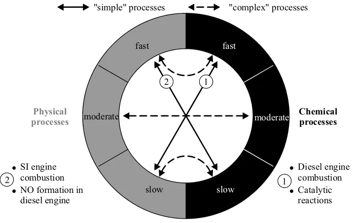
With respect to the simulation of fluid fields with chemical reactions, it should be noted that physical and chemical processes can progress at very different temporal and linear scales. The description of these process progressions is usually simpler when the time scales are much different, because then simplifying assumptions can be made for the chemical or physical process, and it is principally very complex when the time scales are of the same order of mag-nitude. This is made clear by means of the examples in Fig. 1.2.
fast fast
moderate moderate
slow slow
Physical processes
Chemical processes "simple" processes "complex" processes
SI engine combustion NO formation in diesel engine
Diesel engine combustion Catalytic reactions 1
1 2
2
Yet in addition, knowledge of modeling methods is also necessary. Although some universally valid rules can be given for this, this step allows a lot of free room for the creativity and imagination of the modeler. Essentially, the modeling procedure can be subdivided into the following steps:
1st step: define the system and boundaries from the environment, determine the relevant reservoirs as well as the mass and energy flow between them.
2nd step: draw up balance sheets according to the unified scheme: temporal change of the reservoir is equal to the inflow minus the outflow.
3rd step: with the help of physical laws, describe the mass and energy flows.
4th step: simplify the resulting model, if necessary by neglecting secondary influences. 5th step: integrate the model numerically, i.e. execute the simulation.
6th step: validate the model, compare the calculated data with experimentally obtained data. In the utilization of an existing simulation program for the solution of new tasks, the prereq-uisites which were met in the creation of the model must always be examined. It should thereby be clarified whether and to what extent the existing program is actually suitable for the solution of the new problem. One should in such cases always be aware of the fact that "pretty, colorful pictures" exert an enormous power of suggestion upon the "uncritical" ob-server.
The prerequisite for the acceptance of what we nowadays designate as computer simulation was a gradual alteration in philosophical thought and in the conceptualization and understand-ing of the world in which we live. In the past, humanity perceived the world and its processes predominately as linear and causal, and we are gradually comprehending the decisive proc-esses flow in a non-linear and chaotic fashion. Only with the rise of the sciences and with the development of their methodological foundations could the basis for computer simulation be created.
2 Introduction into the functioning of internal
com-bustion engines
2.1 Energy conversion
In energy conversion, we can distinguish hierarchically between general, thermal, and motor energy conversion.
Undergeneral energy conversion is understood the transformation of primary into secondary energy through a technical process in an energy conversion plant, see Fig. 2.1.
Primary energy
Oil derivatives Natural gas
Hydrogen Biomass
Wind Water Sun
E.C.P.
Furnace
internal combustion engine Gas turbine
Fuel cell Power station
Windwheel Hydraulic turbine
Foto cell
Secondary energy
Thermal energy
Mechanical energy
Electric energy
Electric energy
Fig. 2.1: Diagram of general energy conversion
Thermal energy conversion is subject to the laws of thermodynamics and can be described formally, as is shown in Fig. 2.2.
. Qsupplied
Pt
Thermal energy conversion plant
. Qremoved
First law of thermodynamics: P = Q. - Q.
From the second law of thermodynamics follows: .
Q > 0!
Thermal efficiency:
= = 1- < 1
t . remov.
remov.
th
h
suppl
P . Q
t suppl.
. Q
. Q
remov. suppl.
Fig. 2.2: Diagram of thermal energy conversion
the combustion space or chamber, this being then transformed into mechanical energy by the motor. In the case of the stationary gas turbine plant, the mechanical energy is then converted into electrical energy by the secondary generator.
Chemical energy bound in fuel
Thermal energy
Mechanical energy
Electrical energy
Combustion process
Driving mechanism
Generator
Internal combustion
engine Gas turbine
Fig. 2.3: Diagram of energy conversion in an internal combustion engine or gas turbine
2.2 Reciprocating engines
Internal combustion engines are piston machines, whereby one distinguishes, according to the design of the combustion space or the pistons, between reciprocating engines and rotary en-gines with a rotating piston movement. Fig. 2.4 shows principle sketches of possible struc-tural shapes of reciprocating engines, whereby today only variants 1, 2, and 4 are, practically speaking, still being built.
1
2
3 5
4
1 In-line engine 2 V-engine
3 Radial engine 4 Flat engine
Multi-piston units: 5 Dual-piston engine 6 Opposed piston engine 6
2.2 Reciprocating engines 7
For an extensive description of other models of the combustion engine, see Basshuysen and Schäfer (2003) and Maas (1979).
2.2.1 The crankshaft drive
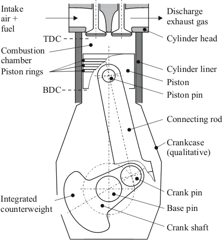
The motor transforms the oscillating movement of the piston into the rotating movement of the crankshaft, see Fig. 2.5. The piston reverses its movement at the top dead center (TDC) and at the bottom dead center (BDC). At both of these dead point positions, the speed of the piston is equal to zero, whilst the acceleration is at the maximum. Between the top dead cen-ter and the underside of the cylinder head, the compression volume Vc remains (also the so-called dead space in the case of reciprocating compressors).
Intake air + fuel
Discharge exhaust gas
TDC
BDC Combustion chamber Piston rings
Integrated counterweight
Cylinder head
Cylinder liner Piston Piston pin
Connecting rod
Crankcase (qualitative)
Crank pin
Base pin
Crank shaft
Fig. 2.5: Assembly of the reciprocating engine
sComp.
c1
e > 0 c2
c3 s ( )j
l
r
j b
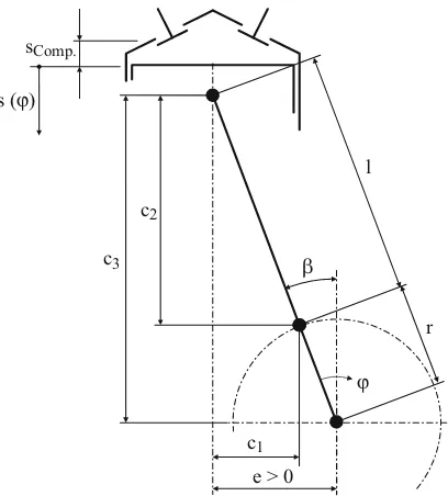
Fig. 2.6: Kinematics of the crankshaft drive
For the piston path s(ϕ), it follows from Fig. 2.6: )
( cos )
(ϕ =c3 −c2 −r ϕ −β
s (2.1)
from which with
2 2 3 2 1 2 2 1 ) ( and , ) ( sin ly respective , sin and sin e l r c c l c r e c l r e arc l r e − + = − = − − = ¸¸ ¹ · ¨¨ © § + = + = ϕ β β β finally
[
sin( )]
cos( )) ( )
(ϕ = r+l 2 −e2 − l2 − e +r ϕ − β 2 −r ϕ −β
s (2.2)
results. The derivative provides for the piston speed the relation
[
]
[
2]
2 sin( )
) ( cos ) ( sin ) ( sin d d β ϕ β ϕ β ϕ β ϕ ϕ − + − − − + + − = r e l r e r r s
. (2.3)
2.2 Reciprocating engines 9
) ( 4 )
(ϕ V D2π s ϕ
V = c + (2.4)
follows for the alteration of cylinder volume
ϕ π ϕ d d 4 d
dV =D2 s .
(2.5) With the eccentric rod relation λe =r l, it follows finally for the limiting case e=0
[
]
¿ ¾ ½ ¯ ® »¼ º «¬ ª − − + −= 1 cos( ) 1 1 1 sin ( )
)
( λ2 2 ϕ
λ ϕ ϕ e e r s (2.6) and » » » ¼ º « « « ¬ ª − + = ) ( sin 1 ) 2 ( sin 2 ) ( sin d d 2 2 ϕ λ ϕ λ ϕ ϕ e e r s . (2.7)
2.2.2 Gas and inertia forces
The motor is driven by the gas pressure p(ϕ) present in the combustion space. With the piston area AP = D2π 4, one then obtains for the gas force
) ( 4
2π p ϕ
D
Fg = . (2.8)
Because of the masses in motion in the driving mechanism, additional and temporally vari-able inertia forces arise, which lead to rotating and oscillating unbalances and must at least partially be counterbalanced in order to guarantee the required driving mechanism running smoothness. The single components of the motor execute rotating (crank pin, mc.p.), oscillat-ing (piston block, mP), or mixed (connecting rod) movements. If one distributes the mass of the connecting rod into a rotating (mc.r.,rot) and an oscillating (mc.r.,osc) portion, one then obtains for the rotating and oscillating masses of the driving mechanism
. , ., . . . ., . p osc r c osc p c rot r c rot m m m m m m + = + =
For small λe, the expression under the root in (2.6) corresponding to
... ) ( sin 8 ) ( sin 2 1 ) ( sin 1 4 4 2 2 2
2 = − − −
−λ ϕ λe ϕ λe ϕ
e
can be developed into a Taylor’s series, whereby the third term for λe =0.25 already be-comes smaller than 000480. and can thus be neglected as a rule. With the help of trigonomet-ric transformations, one finally obtains for the piston path
(
1 cos(2 ))
4) ( cos
1− ϕ + λ − ϕ
= e
r s
. (2.9)
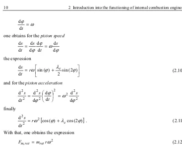
ω ϕ =
t
d d
one obtains for the piston speed
ϕ ω ϕ ϕ d d d d d d d d s t s t s = = the expression » ¼ º « ¬ ª +
= sin(2 )
2 ) ( sin d d ϕ λ ϕ ω e r t s (2.10) and for the piston acceleration
2 2 2 2 2 2 2 2 d d d d d d d d ϕ ω ϕ ϕ s t s t s = ¸ ¹ · ¨ © § = finally
[
cos( ) cos(2 )]
d d 2 2 2 ϕ λ ϕ ω e r t s += . (2.11)
With that, one obtains the expression
2 , m rω
Fmrot = rot (2.12)
for the rotating inertia force, which triggers an unbalance striking in the crankshaft axle and rotating with the speed of the crankshaft. For the oscillating inertia force one obtains the expression
[
cos( ) cos(2 )]
2
,osc osc ω ϕ λe ϕ
m m r
F = + . (2.13)
This consists of two parts, whereby the first rotates with simple crankshaft speed and the second with doubled crankshaft speed. One therefore distinguishes between inertia forces of first and second order,
. ) 2 ( cos , ) ( cos 2 2 2 1 ω λ ω ϕ ω e osc osc r m F r m F = =
The inertia forces are proportional to ω2 and are thus strongly contingent on speed. The resulting piston force consists of gas force and oscillating inertia force,
[
cos( ) cos(2 )]
)( 4
2
2π ϕ ω ϕ λ ϕ
e osc
P D p m r
F = + + . (2.14)
2.2 Reciprocating engines 11
0 180 360 540 720
0 Fm Fg
Pressure Fg
Fm
j[°CA]
Fig. 2.7: Gas force and oscillating inertia force of a 4-stroke reciprocating engine
2.2.3 Procedure
With regard to charge changing in the reciprocating engine, one distinguishes between the 4-stroke and the 2-4-stroke methods and in reference to the combustion process between diesel and spark-ignition (SI) engines. In the case of the 4-stroke-procedure, see also Fig. 2.8, the charge changing occurs in both strokes, expulsion and intake, which is governed by the dis-placement effect of the piston and by the valves. The intake and exhaust valves open before and close after the dead point positions, whereby an early opening of the exhaust valve indeed leads to losses during expansion, but also leads to a diminishment of expulsion work. With increasing valve intersection, the scavenging losses increase, and the operative efficiency decreases. Modern 4-stroke engines are equipped, as a rule, with two intake and two exhaust valves.
p pz
pu
Vc Vd V
IVO EVC
IVC
p pz
pu
Vc Vd V
IVC
4-Stroke-Cycle process 2-Stroke-Cycle process
IVO
EVO EVO
EVC
Fig. 2.8: p,V diagram for the 4-stroke and 2-stroke processes
cylin-der by the in-flowing fresh air, if the piston sweeps over the intake and exhaust sections ar-ranged in the lower area of the cylinder. In the case of larger engines, exhaust valves are mostly used instead of exhaust ports, which are then housed in the cylinder head. Instead of so-called loop scavenging, one then has the fundamentally more effective uniflow scaveng-ing. For more details, see Merker and Gerstle (1997).
2.3 Thermodynamics of the internal combustion engine
2.3.1 Foundations
Our goal in this chapter will be to explain the basic foundations of thermodynamics without going into excessive detail. Extensive presentations can be found in Baehr (2000), Hahne (2000), Lucas (2001), and Stephan and Mayinger (1998, 1999).
For the simulation of combustion-engine processes, the internal combustion engine is sepa-rated into single components or partial systems, which one can principally view either as closed or open thermodynamic systems. For the balancing of these systems, one uses the
mass balance (equation of continuity)
2 1
d d
m m t m
−
= (2.15)
and the energy balance (1st law of thermodynamics)
2 1
d d
E E W Q t
U
+ + +
= (2.16)
with
¸¸ ¹ · ¨¨ © §
+ =
2
2
c h m
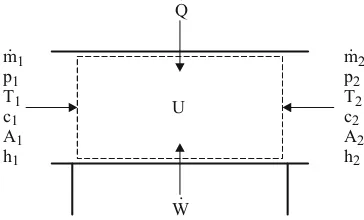
E
for the open, stationary flooded system shown in Fig. 2.9 (flow system), or
W Q t
U
+ =
d d
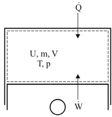
(2.17) for the closed system shown in Fig. 2.10 (combustion chamber).
U
. m p T c A h
2 2
2 2
2 2
. m p T c A h
1 1 1 1 1 1
. Q
. W
2.3 Thermodynamics of the internal combustion engine 13
U, m, V T, p
. Q
. W
Fig. 2.10: Closed thermodynamic system (--- system boundaries)
In closed systems, no mass, and with that no enthalpy, flows over the system limits. Neglect-ing the blow-by losses, the combustion chamber (cylinder) can be viewed as a closed system during the so-called high pressure process (compression and expansion act). In contrast, in the case of an open system, e.g. a reservoir or a line section, masses can flow over the system boundaries.
Neglecting the friction or dissipation of mechanical work into heat, one obtains for the vol-ume work
t V p W
d d
− =
. (2.18)
In the open system, one summarizes the thermal energy transferred to the system boundaries and the intake and expulsion work practically as enthalpy
pv u
h≡ + . (2.19)
Thethermal state equation
0 ) , , (p T v =
f (2.20)
ties together the three thermal condition magnitudes of pressure, temperature, and volume and thecaloric state equation
ly respective ,
) , (
and ) , (
T p h h
v T u u
= =
(2.21) describes the inner energy as a function of temperature and volume, or the enthalpy as a func-tion of pressure and temperature. We will in the following view the materials under considera-tion first as ideal gases, for which the thermal state equation
T R v
p = (2.22)
is applicable. Because the inner energy of ideal gas is only dependent on temperature, follows from (2.19) with (2.22), that this is also valid for enthalpy. Thus for differential alteration of caloric magnitudes of the ideal gas we have:
. ly respective ,
d ) ( d
and d ) ( d
T T c h
T T c u
p v = =
For ideal gas
( )
T c( )
T cR= p − v (2.24)
and
v p c c =
κ (2.25)
are applicable. For reversible condition alterations, the 2nd law of thermodynamics holds in the form
q s
Td =d . (2.26)
With that, it follows from (2.17) with (2.18)
s T v p
u d d
d =− + . (2.27)
With (2.23), it follows for the rise of the isochores of a ideal gas
v
s c
T s
T =
¸ ¹ · ¨ © §
d d
. (2.28)
Analogous to this, it follows for the rise of isobars
p
s c
T s T
= ¸ ¹ · ¨ © §
d d
,
and for the isotherms and isentropes follows
v p v p
− =
d d
or
v p v
p
κ
− =
d d
.
Fig. 2.11 shows the progression of simple state changes in the p,v and T,s diagram.
Isochore
Isobar
Isotherm
Isentrope T
s p
v Isobar Isochore Isentrope Isotherm
Fig. 2.11: Course of a simple change of state in the p, v- and in the T, s diagram
2.3 Thermodynamics of the internal combustion engine 15 t v p t Q t T c m v d d d d d d −
= . (2.29)
Under consideration of the enthalpy flows and the transferred kinetic energy to the system boundaries, one obtains for the energy balance of the open system
¸ ¸ ¹ · ¨ ¨ © § + − ¸ ¸ ¹ · ¨ ¨ © § + + + = + 2 2 d d d d d d d
d 22
2 2 2 1 1 1 c h m c h m t W t Q t m T c t T c
m v v . (2.30)
For stationarily flooded open systems, it follows for the case that no work is transferred
t Q c c h h m d d 2 2 ) ( 2 1 2 2 1 2 = » » ¼ º « « ¬ ª ¸ ¸ ¹ · ¨ ¨ © § − + −
. (2.31)
With this relation, the flow or outflow equation for the calculation of the mass flows through throttle locations or valves can be derived. We consider an outflow process from an infinitely large reservoir and presume that the flow proceeds adiabatically. With the indices "0" for the interior of the reservoir and "1" for the outflow cross section, it follows with c0 =0 from (2.31)
1 0 2 1
2 h h
c
−
= . (2.32)
With the adiabatic relation
κ κ 1 0 1 0 1 − ¸¸ ¹ · ¨¨ © § = p p T T (2.33)
it first follows
» » » ¼ º « « « ¬ ª ¸¸ ¹ · ¨¨ © § − = ¸¸ ¹ · ¨¨ © § − = − κ κ 1 0 1 0 0 1 0 2
1 1 1
2 p p T c T T T c c p p (2.34)
and furthermore for the velocity c1 in the outflow cross section
» » » ¼ º « « « ¬ ª ¸¸ ¹ · ¨¨ © § − − = − κ κ κ κ 1 0 1 0
1 2 1 1
p p T
R
c . (2.35)
With the equation for ideal gas, it follows for the density ratio from (2.33)
κ ρ ρ 1 0 1 0 1 ¸¸ ¹ · ¨¨ © § = p p
. (2.36)
1 1 1 c
A
m = ρ
in the outflow cross section the relation
¸¸ ¹ · ¨¨ © § Ψ = ρ ,κ 0 1 0 0 1 p p p A
m , (2.37)
whereby » » » ¼ º « « « ¬ ª ¸¸ ¹ · ¨¨ © § − ¸¸ ¹ · ¨¨ © § − = ¸¸ ¹ · ¨¨ © § Ψ + κ κ κ κ κ κ 1 0 1 2 0 1 0 1 1 2 , p p p p p p (2.38)
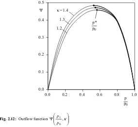
is the so-called outflow function, which is solely contingent upon the pressure ratio p1 p0
and from the isentrope exponent κ. Fig. 2.12 shows the progression of the outflow function for various isentrope exponents.
0.0 0.1 0.2 0.3 0.4 0.5
0.0 0.2 0.4 0.6 0.8 1.0
Y
p p0
p* p0
k= 1.4
1.3
1.2
Fig. 2.12: Outflow function ¸¸
¹ · ¨¨ © § Ψ ,κ 0 1 p p
The maximums of the outflow function result from the relation
max
0 1
for
0 Ψ =Ψ
= ¸¸ ¹ · ¨¨ © § ∂ Ψ ∂ p
2.3 Thermodynamics of the internal combustion engine 17
With this, one obtains for the so-called critical pressure ratio the relation
1 2 or
1 2
0 1 1
0 1
+ = ¸¸ ¹ · ¨¨ © § ¸¸
¹ · ¨¨ © §
+ = ¸¸ ¹ · ¨¨ ©
§ −
κ κ
κ κ
crit
crit T
T p
p
. (2.40)
If we put this relation into (2.35) for the isentropic outflow velocity, then
1 ,
1 RT
c crit = κ (2.41)
finally follows. From (2.36) follows
T R p p
κ ρ κ
ρ = =
d d
(2.42) for the isentropic flow. With the definition of sound speed
ρ d dp
a≡ (2.43)
thus follows
1
1 RT
a = κ (2.44)
for the velocity of the outflow cross section. The flow velocity in the narrowest cross section of a throttle location or in the valve can thereby reach maximal sonic speed.
2.3.2 Closed cycles
The simplest models for the actual engine process are closed, internally reversible cycles with heat supply and removal, which are characterized by the following properties:
- the chemical transformation of fuel as a result of combustion are replaced by a corre-sponding heat supply,
- the charge changing process is replaced by a corresponding heat removal - air, seen as a ideal gas, is chosen as a working medium.
• The Carnot cycle
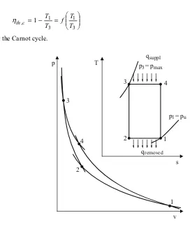
The Carnot cycle, represented in Fig. 2.13, is the cycle with the highest thermal efficiency and thus the ideal process. Heat supply results from a heat bath of temperature T3, heat
re-moval to a heat bath with temperature T1. The compression of 2→3 and 4→1 always
takes place isentropically. With the thermal efficiency
removed supplied
th q
q − =1 η
¸¸ ¹ · ¨¨ © § = − =
3 1 3
1 , 1
T T f T T c
th
η (2.45)
for the Carnot cycle.
p
v 1 2
3
4
p = p3 max
p = p1 u
qsuppl
qremoved
T
s 1 2
3 4
Fig. 2.13: Carnot cycle
The Carnot cycle cannot however be realized in internal combustion engines, because - the isothermal expansion with qsupplied at T3 =const. and the isothermal
compres-sion with qremoved at T1=const. are not practically feasible, and
- the surface in the p,v diagram and thus the internal work is extremely small even at high pressure ratios.
In accordance with the definition, for the medium pressure of the process is applicable
3 1 v
v w pm
−
= . (2.46)
For the supplied and removed heat amounts in isothermal compression and expansion
1 2 1 12
4 3 3 34
ln , ln
p p T R q q
p p T R q q
removed supplied
= =
2.3 Thermodynamics of the internal combustion engine 19
applies. With the thermally and calorically ideal gas, we obtain
1 2 3 2 3 − ¸¸ ¹ · ¨¨ © § = κ κ T T p p
and 1
1 4 1 4 − ¸¸ ¹ · ¨¨ © § = κ κ T T p p
for the isentrope, from which follows
1 4 2 3 p p p p
= and
1 2 4 3 p p p p =
becauseT1 =T2 and T3 =T4. At first we obtain for the medium pressure
3 1
4 3 1 3 )ln
( v v p p T T R pm − − =
and finally by means of simple conversion
1 3 1 3 1 3 1 3 1 3 1 3 1 ln 1 ln 1 T T p p T T p p T T p p p pm − ¸¸ ¹ · ¨¨ © § − − ¸¸ ¹ · ¨¨ © § − = κ κ
. (2.47)
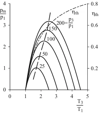
The relation ¸¸ ¹ · ¨¨ © § = , ,κ 1 3 1 3 1 p p T T f p pm
setting to zero and with extreme values is graphically presented in Fig. 2.14 for κ =1,4.
0 1 2 3 4
0 1 2 3 4 5
pm p1 T3 T1 0.2 0.4 0.6 0.8
hth h
th
50
25 100
150 200=pp3
1
While the thermal efficiency in an optimally run process at a pressure ratio of 200 with 0.6 achieves relatively high values, the reachable medium pressure still amounts only to
1
18 .
3 p
pm = . The work to be gained is thus so small that an engine realizing the Carnot cycle could in the best scenario overcome internal friction and can therefore deliver practi-cally no performance.
The Carnot cycle is thus only of interest as a theoretical comparative process. In this context, we can only point out to its fundamental importance in connection to energy considerations.
• The constant-volume process
The constant-volume process is thermodynamically efficient and, in principle, feasible cycle (see Fig. 2.15). In contrast to the Carnot process, it avoids isothermal expansion and compres-sion and the unrealistically high pressure ratio. It consists of two isentropes and two isocho-res. p T v BDC TDC s qremov. qremov.
pmax Tmax
3 4 qsuppl. qsuppl. 2 1 2 1 3 4
Fig. 2.15: Representation of the constant-volume cycle in the p,v and T,s diagram
It is called the constant-volume process because the heat supply (instead of combustion) en-sues in constant space, i.e. under constant volume. Because the piston moves continuously, the heat supply would have to occur infinitely fast, i.e. abruptly. However, that is not realisti-cally feasible. For the thermal efficiency of this process follows
1 1 1 ) ( ) ( 1 1 2 3 1 4 2 1 2 3 1 4 , − − − = − − − = − = T T T T T T T T c T T c q q v v supplied removed v th η .
With the relations for the adiabatic
2.3 Thermodynamics of the internal combustion engine 21
and the compression ratio ε =v1 v2 follows finally for the thermal efficiency of the con-stant-volume process
. 1 1
1 ,
−
¸ ¹ · ¨ © § − =
κ
ε
ηthv (2.48)
This relation, represented in Fig. 2.16, makes it clear that, after a certain compression ratio, no significant increase in the thermal efficiency is achievable.
8
01 4 12 16 20 24
0.0 0.2 0.4 0.6 0.8
hth,V k= 1.4
k= 1.2
e
Fig. 2.16: Efficiency of the constant-volume cycle
• The Constant-pressure process
In the case of high-compressing engines, the compression pressure p2 is already very high. In order not to let the pressure climb any higher, heat supply (instead of combustion) is car-ried out at constant pressure instead of constant volume. The process is thus composed of two isentropes, an isobar, and an isochore, see Fig. 2.17.
p T
v s
qsuppl.
qsuppl.
qremov.
qremov.
pmax
pmax
4
1 2
3
TDC BDC
2
1
4 3 v = const.
Fig. 2.17: The constant-pressure cycle in the p,v and T,s diagram
supplied v supplied removed p th q T T c q
q ( )
1
1 4 1
, = − = − −
η .
As opposed to the constant-volume process, there now appear however three prominent vol-umes. Therefore, a further parameter for the determination of ηth,p is necessary. Pragmati-cally, we select
1 * T c q q p supplied =
for this. With this, we first obtain
¸¸ ¹ · ¨¨ © § − − = − − = 1 * 1 1 * ) ( 1 1 4 1 1 4 , T T q q T c T T c p v p th κ η .
And finally after a few conversions
» » ¼ º « « ¬ ª − ¸¸ ¹ · ¨¨ © § + − =
− 1 1
* * 1 1 1 , κ κ ε κ η q q p
th . (2.49)
The thermal efficiency profile of the constant-pressure process in contingency on ε and *q
is represented in Fig. 2.18.
0 0.1 0.2 0.3 0.4 0.5 0.6 0.7 0.8
0 1 2 4 6 8 10 12 14 16 18 20
Compression ratioe
Thermal ef ficiency hth 1 1 2 2 hth,V hth,p
q* = 4.57
9.14
Fig. 2.18: Thermal efficiency of the constant-pressure cycle
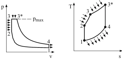
• The Seiliger cycle
2.3 Thermodynamics of the internal combustion engine 23
p
v pmax
3 3*
2
4
T
s 1
2 3
3*
4
1
Fig. 2.19: The Seiliger cycle in the p,v and T,s diagram
One utilizes this comparative process when, at a given compression ratio, the highest pressure must additionally be limited. The heat supply (instead of combustion) succeeds isochorically and isobarically. With the pressure ratio π = p3 p1, we finally obtain the relation
°¿ ° ¾ ½
°¯ ° ®
− ¸ ¹ · ¨ © § » ¼ º «
¬ ª
+ − −
− =
− 1 1
) ( 1 * * 1 1
1 ,
κ κ κ
π ε π ε π ε κ κ
η q
q vp
th (2.50)
for the thermal efficiency, which is graphically represented in Fig. 2.20. From this it becomes clear that, at a constant given compression ratio ε, it is the constant-volume process, and at a constant given pressure ratio π, it is the constant-pressure process which has the highest efficiency.
0 5 10 15 20 25 30
0.2 0.4 0.6 0.8
Constant-pressure Constant-volume
p=100
p=50
p=150
p=200
e 100 50
150 200
0 0.4
0.2 0.3 0.5 0.6 0.7
0.1 0.8
hth hth
30
10 20 e
p
• Comparison of the cycles
p
T
v
s 4
4 1
1 2
2 3
3'
3'
3 3
3
TDC
TDC
BDC
BDC 1
1 2
2 3
3
ε= const. qsuppl= const.
ε= const. qsuppl= const.
v = const. p = const.
v = const. additional q
in the constant-pressure cycle
∆ removed
additional
in the Seiliger cycle
∆removed
Fig. 2.21: Comparison of the closed cycles, ± = constant-volume, ² = constant-pressure, ³ = Seiliger cycle
For the efficiency of t