School of Communications Technology and Mathematical Sciences

School of Communications Technology and Mathematical Sciences

Digital Signal Processing

Part 3

Discrete-Time Signals & Systems

Case Studies

S R Taghizadeh <srt@unl.ac.uk>

Introduction

Matlab and its applications in analysis of continuous-time signals and systems has been discussed in part 1 and 2 of this series of practical manuals. The purpose of part 3 is to discuss the way Matlab is used in analysis of discrete-time signals and systems. Each section provides a series of worked examples followed by a number of investigative problems. You are required to perform each of the worked examples in order to get familiar to the concept of Matlab environment and its important functions. In order to test your understanding of the concept of discrete-time signals & systems analysis, you are required to complete as many of the investigation / case study problems as possible. The areas covered are designed to enforce some of the topics covered in the formal lecture classes. These are:

q Signal Generation and Presentation q Discrete Fourier Transform

q Spectral analysis

Signal Generation and Manipulation

Sinusoidal Signal Generation

Consider generating 64 samples of a sinusoidal signal of frequency 1KHz, with a sampling frequency of 8KHz.

A sampled sinusoid may be written as:

) 2

sin( )

( ₌ p _n+J

f f A

n x

s

where f is the signal frequency, fs is the sampling frequency, q is the phase and A is the amplitude of the signal. The program and its output is shown below:

% Program: W2E1b.m

% Generating 64 samples of x(t)=sin(2*pi*f*t) with a % Frequency of 1KHz, and sampling frequency of 8KHz.

N=64; % Define Number of samples

n=0:N-1; % Define vector n=0,1,2,3,...62,63

f=1000; % Define the frequency

fs=8000; % Define the sampling frequency

x=sin(2*pi*(f/fs)*n); % Generate x(t)

plot(n,x); % Plot x(t) vs. t

grid;

title('Sinewave [f=1KHz, fs=8KHz]'); xlabel('Sample Number');

ylabel('Amplitude');

0 10 20 30 40 50 60 70

-1 -0.8 -0.6 -0.4 -0.2 0 0.2 0.4 0.6 0.8 1

Sinewave [f=1KHz, fs=8KHz]

Sample Number

A

m

pl

it

Note that there are 64 samples with sampling frequency of 8000Hz or sampling time of 0.125 mS (i.e. 1/8000). Hence the record length of the signal is 64x0.125=8mS. There are exactly 8 cycles of sinewave, indicating that the period of one cycle is 1mS which means that the signal frequency is 1KHz.

Task: Generate the following signals

(i) 64 Samples of a cosine wave of frequency 25Hz , sampling frequency 400Hz, amplitude of 1.5 volts and phase =0.

(ii) The same signal as in (i) but with a phase angle of p_{/4 (i.e. 45}o_).

Exercise 2: Exponential Signal Generation

Generating the signal x₍t₎ e 0.1t for t _{0 to 40}mS _{in steps of 0.1}mS =

=

-% Program W2E2.m

% Generating the signal x(t)=exp(-0.1t)

t=0:0.1:40; x=exp(-0.1*t); plot(t,x); grid;

title('Exponential Signal'); xlabel('Time [mS]');

ylabel('Amplitude');

And the output is:

0 5 10 15 20 25 30 35 40

0 0.1 0.2 0.3 0.4 0.5 0.6 0.7 0.8 0.9 1

Exponential Signal

Time [mS]

A

m

p

lit

u

d

Task: Generate the signal: _x(_t)_=e-0.1tsin(0.6_t) for t ₌0 to40msin stepsof 0.1Sec

Exercise 3: Unit Impulse Signal Generation

An impulse is defined as follows:

î í

ì =

=

elsewhere n n

0

0 1

) ( d

The following Matlab program generates a unit impulse signal.

% Program W2E3.m

% Generating 64 Samples of a unit impulse signal

N=64; % Define the number of samples

n=-(N/2):((N/2)-1); % Define a vector of sample numbers

x=zeros(1,N); % Define a vector of zeros

x((N/2)+1)=1.0; % Make the first sample to be 1 (i.e.at t=0)

plot(n,x); % Plot the impulse

grid;

title('A Unit Impulse Signal'); xlabel('Sample Number');

ylabel('Amplitude');

-40 -30 -20 -10 0 10 20 30 40

0 0.1 0.2 0.3 0.4 0.5 0.6 0.7 0.8 0.9 1

A Unit Impulse Signal

Sample Number

A

m

p

lit

u

d

e

Task: Generate 40 samples of the following signals: (for n=-20,-19,-18,…,0,1,2,3,…,18,19) (i) x(n)=2d_(n-10)

(ii) x(n)=5d_(n-10)+2.5d_(n-20)

Exercise 4: Unit Step Signal Generation

A step signal is defined as follows:

î í

ì ³

=

otherwise n n

u

0

0 1

) (

The following Matlab Program generates and plots a unit step signal:

% Program: W2E4.m

% Generates 40 samples of a unit step signal, u(n)

N=40; % Define the number of samples

n=-20:20; % Define a suitable discrete time axis

u=[zeros(1,(N/2)+1),ones(1,(N/2))]; % Generate the signal

plot(n,u); % Plot the signal

axis([-20,+20,-0.5,1.5]); % Scale axis grid;

title('A Unit Step Signal'); xlabel('Sample Number'); ylabel('Amplitude');

-20 -15 -10 -5 0 5 10 15 20

-0.5 0 0.5 1 1.5

A Unit Step Signal

Sample Number

A

m

pl

it

ud

Task: Generate 40 samples of each of the following signals using an appropriate discrete time scale:

(i) x(n)=u(n)-u(n-1) (ii) g(n)=u(n-1)-u(n-5)

Exercise 5: Generating Random Signals

Random number generators are useful in signal processing for testing and evaluating various signal processing algorithms. For example, in order to simulate a particular noise cancellation algorithm (technique), we need to create some signals which is contaminated by noise and then apply this signal to the algorithm and monitor its output. The input/ output spectrum may then be used to examine and measure the performance of noise canceller algorithm. Random numbers are generated to represent the samples of some noise signal which is then added to the samples of some the wanted signal to create an overall noisy signal. The situation is demonstrated by the following diagram.

Matlab provides two commands, which may be applied to generate random numbers.

Normally Distributed Random Numbers. randn(N)

Is an N-by-N matrix with random entries, chosen from a normal distribution with mean zero and variance one.

randn(M,N), and randn([M,N]) are M-by-N matrices with random entries.

S

+ +

Output, s(n)=x(n)+w(n)

Input, x(n)

Noise, w(n)

Noise Cancellation

algorithm

Uniformly Distributed Random Numbers.

rand(N) is an N-by-N matrix with random entries, chosen from a uniform

distribution on the interval (0.0,1.0).

rand(M,N) and rand([M,N]) are M-by-N matrices with random entries.

The following Matlab program generates random signals using each distribution.

% Program: W2E5.m

% Generates Uniformly and Normally Distributed random signals

N=1024; % Define Number of samples

R1=randn(1,N); % Generate Normal Random Numbers

R2=rand(1,N); % Generate Uniformly Random Numbers

figure(1); % Select the figure

subplot(2,2,1); % Subdivide the figure into 4 quadrants

plot(R1); % Plot R1 in the first quadrant

grid;

title('Normal [Gaussian] Distributed Random Signal'); xlabel('Sample Number');

ylabel('Amplitude');

subplot(2,2,2); % Select the second qudrant

hist(R1); % Plot the histogram of R1

grid;

title('Histogram [Pdf] of a normal Random Signal'); xlabel('Sample Number');

ylabel('Total');

subplot(2,2,3); plot(R2);

grid;

title('Uniformly Distributed Random Signal'); xlabel('Sample Number');

ylabel('Amplitude');

subplot(2,2,4); hist(R2);

grid;

title('Histogram [Pdf] of a uniformly Random Signal'); xlabel('Sample Number');

Task: Generate 128 Uniformly random numbers between -p _{to +}p

Exercise 6: Signal Manipulation

Some of the basic signal manipulation may be listed as follows:

v Signal Shifting / Delay

Here 'D' is the number of samples which the input signal must be delayed. For example if x(n)=[1, 2, 3, 4, 5], then x(n-3)=[0,0,0,1,2,3,4,5].

0 200 400 600 800 1000 1200 -4

-2 0 2 4

Normal [Gaussian] Distributed Random Signal

Sample Number

A

m

pl

it

ude

-4 -2 0 2 4

0 50 100 150 200 250 300

Histogram [Pdf] of a normal Random Signal

Sample Number

To

ta

l

0 200 400 600 800 1000 1200 0

0.2 0.4 0.6 0.8 1

Uniformly Distributed Random Signal

Sample Number

A

m

pl

it

ude

0 0.2 0.4 0.6 0.8 1 0

50 100 150

Histogram [Pdf] of a uniformly Random Signal

Sample Number

To

ta

l

D Z

v Signal Addition / Subtraction

When adding two signals together, signals must have the same number of samples. If one signal has less than number of samples than the other, then this signal may be appended with zeros in order to make it equal length to the second signal before

adding them.

v Signal Amplification / Attenuation

'a' is a numerical constant. If a>1, then the process is referred to as 'amplification' , if 0<a<1, the process is referred to as 'attenuation'.

v Signal Differentiation / Integration a

S

+ +

Output, y(n)=x1(n)+x2(n)

Input, x1(n)

Input, x2(n)

Input, x1(n) Output,

y(n)=ax(n)

atin Differenti dt

d

Input, x(t) Output,

) ( )

( x t

dt d n

y ₌

n Integratio

ò

Input, x(t) Output,

dt t x n y

t

t

ò

=

2

v Signal Multiplication / Division

A Matlab program given below, provide an example of each of the above basic operations:

% Program: W2E6.m

% Program demonstrating Basic Signal Manipulation

N=128; f1=150; f2=450; f3=1500; fs=8000; n=0:N-1;

x1=sin(2*pi*(f1/fs)*n);

x2=(1/3)*sin(2*pi*(f2/fs)*n); x3=sin(2*pi*(f3/fs)*n);

figure(1);

subplot(1,1,1); subplot(2,3,1); plot(n,x1); grid;

title('Signal, x1(n)');

subplot(2,3,2); plot(n,x2); grid;

title('Signal, x2(n)');

subplot(2,3,3); plot(n,x3); grid;

title('Signal, x3(n)');

% Signal Delay

x1d=[zeros(1,20), x1(1:N-20)]; subplot(2,3,4);

plot(n,x1d);

X

+ +

Output, y(n)=x1(n)*x2(n)

Input, x1(n)

grid;

title('Delayed x(n), [x1(n-20)]');

% Signal Addition

xadd=x1+x2; subplot(2,3,5); plot(n,xadd); grid;

title('x1(n)+x2(n)');

% Signal Multiplication

xmult=x1.*x3; subplot(2,3,6); plot(xmult); grid;

title('x1*x3');

0 100 200 -1

-0.5 0 0.5 1

Signal, x1(n)

0 100 200 -0.4

-0.2 0 0.2 0.4

Signal, x2(n)

0 100 200 -1

-0.5 0 0.5 1

Signal, x3(n)

0 100 200 -1

-0.5 0 0.5 1

Delayed x(n), [x1(n-20)]

0 100 200 -1

-0.5 0 0.5 1

x1(n)+x2(n)

0 100 200 -1

-0.5 0 0.5 1

Discrete Fourier Transform

[1] Given a sampled signal x(n), its Discrete Fourier Transform (DFT) is given by:

å

-=

-=

1 0 2 N n N / nk j

e

)

n

(

x

)

k

(

X

p k=0,1,2,…,N-1

The magnitude of the X(k) [i.e. the absolute value] against k is called the spectrum of x(n). The values of k is proportional to the frequency of the signal according to:

N

kF

f

_k

=

s

Where Fs is the sampling frequency.

Assuming x is the samples of the signal of length N, then a simple Matlab program to perform the above sum is shown below:

n=[0:1:N-1]; k=[0:1:N-1];

WN=exp(-j*2*pi/N); nk=n'*k;

WNnk=WN .^ nk; Xk=x * WNnk;

Use the above routine to determine and plot the DFT of the following signal:

)

t

f

cos(

)

t

f

cos(

)

t

(

x

=

2

p

₁

+

2

p

₂

where

128

N

and

,

Hz

F

with

,

Hz

f

and

Hz

f

₁

=

1000

₂

=

400

_s

=

8000

=

Note: Plot the magnitude and phase of Xk as follows:

MagX=abs(Xk);

subplo(2,1,1); plot(k,MagX); subplot(2,1,2); plot(k,PhaseX);

Investigate:

(i) At what value of the index k does the magnitude of the DFT of x has major peaks.

(ii) What is the corresponding frequency of the two peaks. (iii) Perform the above for N=32, 64 and 512.

(iv) Comment on the results

(v) Set 128 and generate x(n) for n=0,1,2,…,N-1. Append a further 512 zeros to x(n) as shown below: [Note the number of samples, N=128+512=640].

Xe=[x, zeros(1,512)];

Perform the DFT of the new sequence and plot its magnitude and phase. Compare with the previous result. Explain the effect of zero padding a signal with zero before taking the discrete Fourier Transform.

[2] Inverse DFT is defined as:

1 -N n 0 for )

( 1 ) (

1

0

/ 2

£ £ =

å

-=

N

k

N nk j e k X N n

x p

A simple Matlab routine to perform the inverse DFT may be written as follows:

n=[0:1:N-1]; k=[0:1:N-1];

WN=exp(-j*2*pi/N); nk=n'*k;

Use x(n)={1,1,1,1}, and N=4, determine the DFT. Record the Magnitude and phase of the DFT.

Use the IDFT to transfer the DFT results (i.e. Xk sequence) to its original sequence.

Spectral Analysis of a signal

Let

x

(

t

)

=

cos(

2

p

f

₀

t

)

where

f

₀

=

30

Hz

, assuming the sampling frequency

samples

256

N

and

Hz

f

_s

=

128

=

, obtain the FFT of the windowed signal using rectangular and hamming windows, zero padded to N1=1024. Plot the normalised FFT magnitude of the windowed signals. Which windowed signal shows a narrower mainlobe?. Which windowed signal shows the smaller peak sidelobe?.

A Matlab program implementing the spectrum is shown below:

f1=30; % Signal frequency

fs=128; % Sampling frequency

N=256; % Number of samples

N1=1024; % Number of FFT points

n=0:N-1; % Index n

f=(0:N1-1)*fs/N1; % Defining the frequency points [axis]

x=cos(2*pi*f1*n/fs); % Generate the signal

XR=abs(fft(x,N1)); % find the magnitude of the FFT using No % windowing (i.e. Rectangular window)

xh=hamming(N); % Define the hamming samples

xw=x .* xh'; % Window the signal

XH=abs(fft(xw,N1)); % find the magnitude of the FFT of the % windowed signal.

subplot(2,1,1); % Start plotting the signal

plot(f(1:N1/2),20*log10(XR(1:N1/2)/max(XR)));

title('Spectrum of x(t) using Rectangular Windows'); grid;

xlabel('Frequency, Hz');

ylabel('Normalised Magnitude, [dB]'); subplot(2,1,2);

plot(f(1:N1/2),20*log10(XH(1:N1/2)/max(XH))); title('Spectrum of x(t) using Hamming Windows'); grid;

xlabel('Frequency, Hz');

And here is the output from the program:

It can be seen from the spectrum plots that both the rectangular window and hamming window have their peak amplitude at f=30Hz corresponding to the signal frequency. While the rectangular window has a narrower mainlobe, hamming window provides less peak sidelobes than the rectangular window. There are many other types of windows which are available as Matlab functions and are listed below:

bartlett(N) returns the N-point Bartlett window blackman(N) returns the N-point Blackman window boxcar(N) returns the N-point rectangular window hamming(N) returns the N-point Hamming window.

hanning(N) returns the N-point Hanning window in a column vector. kaiser(N,beta) returns the BETA-valued N-point Kaiser window. triang(N) returns the N-point triangular window.

Further Spectral Analysis

The spectrum of a signal is simply a plot of the magnitude of the components of a signal against their corresponding frequencies. For example if a signal consists of two

0 10 20 30 40 50 60 70

-400 -300 -200 -100 0

Spectrum of x(t) using Rectangular Windows

Frequency, Hz

N

o

rm

al

is

ed M

agni

tu

de,

[

dB

]

0 10 20 30 40 50 60 70

-150 -100 -50 0

Spectrum of x(t) using Hamming Windows

Frequency, Hz

N

o

rm

al

is

ed M

a

gni

tu

de,

[

dB

sinusoidal at 120Hz and 60Hz, then ideally the spectrum would be a plot of magnitude vs. frequency and would contain two peaks: one at 60 Hz and the other at 120 Hz illustrated in the next example. The following Matlab commands are the basis of determining the spectrum of a signal:

fft

psd

spectrum

In the following examples, we illustrate their use. One of the most important aspects of spectral analysis is the interpretation of the spectrum and its relation to the signal under investigation.

Task 1:

Generate 256 samples of a sinusoidal signal of frequency 1KHz with a sampling frequency of 8KHz. Plot the signal and its spectrum.

Here is the program:

N=256; % Total Number of Samples

fs=8000; % Sampling frequency set at 1000Hz

f=1000; n=0:N-1;

% Now generate the sinusoidal signal

x=sin(2*pi*(f/fs)*n);

% Estimate its spectrum using fft command

X=fft(x); magX=abs(X);

% Build up an appropriate frequency axis

fx=0:(N/2)-1; % first make a vector for f=0,1,2,...(N/2)-1

fx=(fx*fs)/N; % Now scale it so that it represents frequencies in Hz

figure(1);

subplot(1,1,1);

plot(fx,20*log10(magX(1:N/2))); grid;

title('Spectrum of a sinusoidal signal with f=1KHz'); xlabel('Frequency (Hz)');

And the output:

It is clear from the spectrum, that the signal consists of a single sinusoidal components of frequency 1000Hz. Other artefacts in the figure are due to the limited number of samples, windowing effects, and computation accuracy.

Task 1:

Consider, the notch filter in the previous section. The transfer function of the notch filter is repeated here for convenience:

0 1000 2000 3000 4000 -350

-300 -250 -200 -150 -100 -50 0 50

Spectrum of a sinusoidal signal with f=1KHz

Frequency (Hz)

M

ag

ni

tud

e (

dB

Apply an input signal: ) 2 sin( ) 2 sin( )

( 1 2

s s f n f f n f n

x ₌ p ₊ p , with f1=120 Hz , f2=60 Hz and fs , the

sampling frequency at 1000Hz.

Plot the followings:

Input Spectrum

Magnitude response of the filter Output Spectrum

Here is the Matlab Program:

% Program Name: Tut16.m

clear;

N=1024; % Total Number of Samples

fs=1000; % Sampling frequency set at 1000Hz

f1=120; f2=60; n=0:N-1; x=sin(2*pi*(f1/fs)*n)+sin(2*pi*(f2/fs)*n); [pxx,fx]=psd(x,2*N,fs); plot(fx,20*log10(pxx)); grid;

title('Magnitude Spectrum of x(n)'); xlabel('Frequency, Hz');

ylabel('Magnitude, dB'); sin(2*pi*(f2/fs)*n); b=[1 -1.8596 1];

a=[1 -1.8537 0.9937]; k=0.9969; b=k*b; figure(1); subplot(1,1,1); subplot(1,3,1); Output, y(n) Input, x(n) 2 1 2 1

9937

.

0

8537

.

1

1

8996

.

1

1

9969

.

0

)

(

-+

-+

-=

z

z

z

z

z

H

[pxx,fx]=psd(x,2*N,fs); plot(fx,20*log10(pxx)); grid;

title('Magnitude Spectrum of x(n)'); xlabel('Frequency, Hz');

ylabel('Magnitude, dB');

[h,f]=freqz(b,a,1024,fs); % Determines the frequency response % of

% the filter with coefficients 'b' % and 'a', using 1024 points around % the unit circle with a sampling

% frequency of fs. The function % returns the values of the transfer % function h, for each frequency in

% f in Hz.

magH=abs(h); % Calculates the magnitude of the filter

phaseH=angle(h); % Calculates the phase angle of the filter

subplot(1,3,2); % Divides the figure into two rows and one

% column and makes the first row the active

% one

plot( f, 20*log10(magH)); % plots the magnitude in dB against

% frequency

grid; % Add a grid

title('Magnitude Response of the Notch Filter'); xlabel('Frequency');

ylabel('Magnitude, dB');

y=filter(b,a,x);

[pyy,fy]=psd(y,2*N,fs); % determine the Spectrum using 'psd'

subplot(1,3,3); % Select the third column in the figure

plot(fy,20*log10(pyy)); % Plot the output spectrum in dB

grid; % Add a grid

title('Magnitude Spectrum of y(n)'); xlabel('Frequency, Hz');

ylabel('Magnitude, dB');

It can be seen from the plot, that the input signal consists of two sinusoidal components at 60Hz and 120Hz. From the magnitude response of the filter, it is clear that the filter attenuates components whose frequencies are at 60 Hz. Therefore, the output spectrum consists of the 120 Hz signal and attenuated (0 dB) signal at 60Hz.

A final example considers the use of the Matlab command 'spectrum' in order to estimate the spectrum of a given signal.

Task 3:

Consider estimating the spectrum of a signal consisting of three sinusoidal signals at frequencies, f1=500Hz, f2=1000Hz, and f3=1500Hz. Assume a sampling frequency of 8KHz.

The Matlab Program and its output is shown next: % Program Name: Tut17.m

clear;

N=1024; % Total Number of Samples

fs=8000;% Sampling frequency set at 1000Hz

f1=500; f2=1000; f3=1500; n=0:N-1;

0 200 400 600 -100 -80 -60 -40 -20 0 20 40

Magnitude Spectrum of x(n)

Frequency, Hz

Magn

it

ude,

dB

0 200 400 600 -18 -16 -14 -12 -10 -8 -6 -4 -2 0 2

Magnitude Response of the Notch Filter

Frequency

Magn

it

ude,

dB

0 200 400 600 -80 -60 -40 -20 0 20 40

Magnitude Spectrum of y(n)

Frequency, Hz

Magn

it

ude,

x=sin(2*pi*(f1/fs)*n)+sin(2*pi*(f2/fs)*n)+sin(2*pi*(f3/fs)*n); pxx=spectrum(x,N); % Estimate the Spectrum

specplot(pxx,fs); % Plot the spectrum grid;

title('Power Spectrum of x(n)'); xlabel('Frequency, Hz');

ylabel('Magnitude, dB');

And the output:

0 500 1000 1500 2000 2500 3000 3500 4000 10-15

10-10 10-5 100 105

Power Spectrum of x(n)

Frequency, Hz

M

agni

tude,

d

Autocorrelation and Crosscorrelation in Matlab

Both in signal and Systems analysis, the concept of autocorrelation and crosscorrelation play an important role. In the following sections, we present some simple examples of how these two functions may be estimated in Matlab. The final part of this section provides some applications of autocorrelation and crosscorrelation functions in signal detection and time-delay estimations.

The autocorrelation function of a random signal describes the general dependence of the values of the samples at one time on the values of the samples at another time. Consider a random process x(t) (i.e. continuous-time), its autocorrelation function is written as:

ò

-¥ ®

+

=

T T T

xx

x

(

t

)

x

(

t

)

dt

T

lim

)

(

R

t

t

2

1

(1)

Where T is the period of observation.

)

(

R

_xx

t

is always real-valued and an even function with a maximum value at

t

=

0

.

For sampled signal (i.e. sampled signal), the autocorrelation is defined as either biased or unbiased defined as follows:

where M is the number of lags.

Some of its properties are listed in table 1.1.

The cross correlation function however measures the dependence of the values of one signal on another signal. For two WSS (Wide Sense Stationary) processes x(t) and y(t) it is described by:

ò

-¥

®

+

=

T

T T

xy

x

(

t

)

y

(

t

)

dt

T

lim

)

(

R

t

1

t

(3)

or

ò

-¥

®

+

=

T

T T

yx

y

(

t

)

x

(

t

)

dt

T

lim

)

(

R

t

1

t

(4)

where T is the observation time.

For sampled signals, it is defined as:

å

- +

=

-+

=

1

1

1

1

N m

n

yx

y

(

n

)

x

(

n

m

)

N

)

m

(

R

(5)

m=1,2,3,..,N+1

Where N is the record length (i.e. number of samples).

Autocorrelation Properties

[1] Maximum Value:

The magnitude of the autocorrelation function of a wide sense stationary random process at lag m is upper bounded by its value at lag m=0:

0

k

for

)

k

(

R

)

(

R

_xx

0

³

_xx

¹

[2] Periodicity:

If the autocorrelation function of a WSS random process is such that:

)

(

R

)

m

(

R

_{xx 0}

=

_xx

0

for some

m

₀, then

R

_xx

(

m

)

is periodic with period

m

₀.

Furthermore

E

[

x

(

n

)

-

x

(

n

-

m

₀

)

2

]

=

0

and x(n) is said to be mean-square

periodic.

[3] The autocorrelation function of a periodic signal is also periodic:

Example: if

x

(

n

)

=

A

sin(

w

₀

n

+

j

)

, then,

R

_xx

(

m

)

A

cos(

₀

m

)

2

2

w

=

Therefore if

,

then

R

(

m

)

N

xx

p

w

2

0

=

is periodic with periodic N and x(n) is

mean-square periodic.

[4] Symmetry:

The autocorrelation function of WSS process is a conjugate symmetric function of m:

)

m

(

R

)

m

(

R

_xx

=

*_xx

-For a real process, the autocorrelation sunction is symmetric:

R

_xx

(

m

)

=

R

_xx

(

-

m

)

[5] Mean Square Value:

{

}

0

0

)

=

E

x

(

n

)

2

³

(

R

_xx

[6] If two random processes x(n) and y(n) are uncorrelated, then the autocorrelation of the sum x(n)=s(n)+w(n) is equal to the sum of the autocorrelations of s(n) and w(n):

)

m

(

R

)

m

(

R

)

m

(

R

_xx

=

_ss

+

_ww

[7] The mean value:

The mean or average value (or d.c.) value of a WSS process is given by:

)

(

R

x

,

mean

=

_xx

¥

Table 1.1 Properties of Autocorrelation function

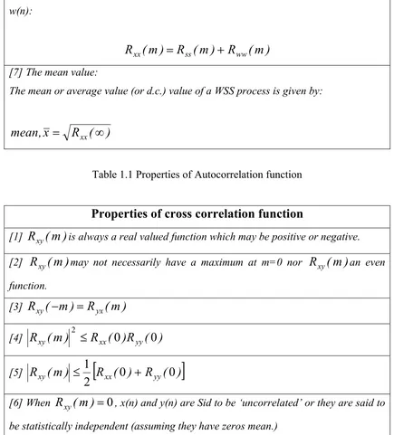
Properties of cross correlation function

[1]

R

_xy

(

m

)

is always a real valued function which may be positive or negative.

[2]

R

_xy

(

m

)

may not necessarily have a maximum at m=0 nor

R

_xy

(

m

)

an even

function.

[3]

R

_xy

(

-

m

)

=

R

_yx

(

m

)

[4]

R

_xy

(

m

)

2

£

R

_xx

(

0

)

R

_yy

(

0

)

[5]

R

_xy

(

m

)

[

R

_xx

(

0

)

R

_yy

(

0

)

]

2

1

+

£

[6] When

R

_xy

(

m

)

=

0

, x(n) and y(n) are Sid to be ‘uncorrelated’ or they are said to

be statistically independent (assuming they have zeros mean.)

Matlab Implementation

Matlab provides a function called xcorr.m which may be used to implement both auto and cross correlation function. Its use is indicated in the following examples:

Example 1: Autocorrelation of a sinewave

Plot the autocorrelation sequence of a sinewave with frequency 1 Hz, sampling frequency of 200 Hz.

The Matlab program is listed below:

N=1024; % Number of samples

f1=1; % Frequency of the sinewave FS=200; % Sampling Frequency

n=0:N-1; % Sample index numbers

x=sin(2*pi*f1*n/FS); % Generate the signal, x(n) t=[1:N]*(1/FS); % Prepare a time axis

subplot(2,1,1); % Prepare the figure plot(t,x); % Plot x(n)

title('Sinwave of frequency 1000Hz [FS=8000Hz]'); xlabel('Time, [s]');

ylabel('Amplitude'); grid;

Rxx=xcorr(x); % Estimate its autocorrelation subplot(2,1,2); % Prepare the figure

plot(Rxx); % Plot the autocorrelation grid;

title('Autocorrelation function of the sinewave'); xlable('lags');

ylabel('Autocorrelation');

The output of this program is shown next.

Note that if you want to write your own autocorrelation function, you may use equation (2) to do this. Here is a how it may be written:

function [Rxx]=autom(x) % [Rxx]=autom(x)

% This function Estimates the autocorrelation of the sequence of

% random variables given in x as: Rxx(1), Rxx(2),…,Rxx(N), where N is

% Number of samples in x.

N=length(x); Rxx=zeros(1,N);

for m=1: N+1

for n=1: N-m+1

Rxx(m)=Rxx(m)+x(n)*x(n+m-1);

end;

end;

0 1 2 3 4 5 6

-1 -0.5 0 0.5 1

Sinwave of frequency 1000Hz [FS=8000Hz]

Time, [s]

A

m

p

lit

u

d

e

0 500 1000 1500 2000 2500

-500 0 500 1000

Autocorrelation function of the sinewave

lags

A

u

to

co

rr

e

la

ti

o

To use the above function, you need to save this under autom.m and then it may be used as follows:

N=1024; f1=1; FS=200; n=0:N-1;

x=sin(2*pi*f1*n/FS); t=[1:N]*(1/FS);

subplot(2,1,1); plot(t,x);

title('Sinwave of frequency 1000Hz [FS=8000Hz]'); xlabel('Time, [s]');

ylabel('Amplitude'); grid;

Rxx=autom(x); subplot(2,1,2); plot(Rxx);

grid;

title('Autocorrelation function of the sinewave'); xlabel('lags');

ylabel('Autocorrelation');

Example 2: Crosscorrelation

Plot the crosscorrelation of the following signal:

)

n

(

w

)

n

(

x

)

n

(

y

Hz

f

with

)

t

f

sin(

)

n

(

x

₁

+

=

=

=

2

p

1

1

where w(n) is a zeros mean, unit variance of Gaussina random process.

N=1024; % Number of samples to generate f=1; % Frequency of the sinewave FS=200; % Sampling frequency

n=0:N-1; % Sampling index x=sin(2*pi*f1*n/FS); % Generate x(n) y=x+10*randn(1,N); % Generate y(n) subplot(3,1,1);

plot(x);

title('Pure Sinewave'); grid;

subplot(3,1,2);

0 1 2 3 4 5 6

-1 -0.5 0 0.5 1

Sinwave of frequency 1000Hz [FS=8000Hz]

Time, [s] Am p lit u d e

0 200 400 600 800 1000 1200

-600 -400 -200 0 200 400 600

Autocorrelation function of the sinewave

plot(y);

title('y(n), Pure Sinewave + Noise'); grid;

Rxy=xcorr(x,y); % Estimate the cross correlation subplot(3,1,3);

plot(Rxy);

title('Cross correlation Rxy');

grid;

The output is:

0 200 400 600 800 1000 1200

-1 -0.5 0 0.5 1

Pure Sinewave

0 200 400 600 800 1000 1200

-40 -20 0 20 40

y(n), Pure Sinewave + Noise

0 500 1000 1500 2000 2500

-500 0 500

Question [1]

From the results shown for example 2, what function cross correlation has performed.

Question [2]

Given

x

(

n

)

=

A

sin(

w

t

+

J

)

0 , prove that its autocorrelation function is given by:

)

cos(

A

)

(

R

_xx

t

wt

2

2

=

Case Study

Time Delay Estimation

Processing Radar Returned Signal

Consider a simple radar illustration shown below:

A pulse x(t) is transmitted, the reflected signal from an object is returned to the receiver. The returned signal (r(t)) is delayed (i.e. D seconds) , noisy and attenuated. The objective is to measure (estimate) the time delay between the transmitted and the returned signal.

Analysis: Let the transmitted signal be x(t), then the returned signal r(t) may be modelled as:

)

t

(

w

)

D

t

(

x

)

t

(

r

=

a

-

+

The Target

Returned signal, r(t) Transmitted signal, x(t)

)

t

(

w

)

D

t

(

x

)

t

(

r

=

a

-

+

where: w(t) is assumed to be the additive noise during the transmission.

a

is the attenuation factor (<1).

D is the delay which is the time taken for the signal to travel from the transmitter to the target and back to the receiver.

A common method of estimating the time delay D is to compute the cross-correlation function of the received signal with the transmitted signal x(t). i.e.

{

}

[

][

]

{

}

{

}

)

(

R

)

D

(

R

)

(

R

Hence

)

w(t)x(t

)

D)x(t

-x(t

E

)

t

(

x

w(t)

D)

-x(t

E

)

t

(

x

)

t

(

r

E

)

(

R

wx xx rx rx

t

t

a

t

t

t

a

t

a

t

t

+

-=

+

+

+

=

+

+

=

+

=

(6)

Note, ‘E’ is the expectation operator.

Therefore, the cross correlation

R

_rx

(

t

)

_{is equal to the sum of the scaled}

autocorrelation function of the transmitted signal (i.e.

a

R

_xx

(

t

)

) and the cross

correlation function between x(t) and the contaminated noise signal w(t). If we now assume that the noise signal w(t) and the transmitted signal x(t) are uncorrelated then,

0

=

)

(

R

_wx

t

This is also stated in table 1.2 under the property number [6].

Hence the cross-correlation function between the transmitted signal and the received signal may be written as:

)

D

(

R

)

(

Therefore if we plot

R

_rx

(

t

)

_{, it will only have one peak value that will occur at}

D

=

t

. A typical plot of

R

(

)

rx

t

is shown below:

Investigation

[1] Generate a single pulse for the transmitted signal as shown below:

0 50 100 150 200 250 300

-100 -50 0 50 100 150 200 250 300 350

Crosscorrelation Rrx

Estimated Time Delay as number of

samples

x(n)

0 N=256

5

[2] Delay the signal by say 32 samples and reduce its amplitude by an attenuation factor of say

a

=

0.

7

, call this xd(n) as shown below:

[3] Generate N=256 samples of Gaussian random signal and call this w(n).

[4] Generate the simulated received signal by adding the transmitted signal x(n) and the noise signal w(n), i.e.

)

n

(

w

sigman

)

d

n

(

x

)

n

(

r

=

a

-

+

´

Where sigman is the noise amplitude (initially set this to 1.

[5] using subplot(2,2,1), plot the signals x(n), xd(n), and r(n). Appropriately label and grid the each plot.

[6] Estimate the cross-correlation sequence

R

_rx

(

m

)

and plot in the fourth quadrant of the figure. Note , plot only half the samples of the cross correlation sequence returned by the function xcorr. This can be done as follows:

% Assuming there are N samples of x Y=xcorr(r,x);

R=Y(1:N); Rrx=fliplr(R); .

.

xd(n)

0 N=256

5a

[7] From the plot estimate the delay. Does it agree with the theoretical delay value?

[8] Repeat the simulation for some values of

a

, sigman, and N?

[9] Comment on your findings?

Time delay Estimation in Frequency Domain

Consider the returned signal once again:

)

t

(

w

)

D

t

(

x

)

t

(

r

=

a

-

+

Taking the Fourier transform of both sides yields:

)

(

W

e

)

(

X

)

(

P

_r

w

=

a

w

-jwD

+

w

Or taking the Fourier Transform of the cross correlation of r(t) and x(t) gives:

)

(

P

e

)

(

P

)

(

P

_rx

w

=

a

_xx

w

-jwD

+

_wx

w

Assuming that the transmitted signal and the contaminated noise are uncorrelated, we get:

D j xx

xr

(

)

P

(

)

e

P

w

w

a

w

=

-Therefore by having an estimate of the cross spectral function of the transmitted and the received signal, we can estimate the time delay from its phase:

fD

2

D

Phase

p

w

Hence by taking the slope of the phase (i.e.

Phase

)

f

(

d

d

), we have the slope of the

phase which may be written as:

p

p

2

2

Slope

D

Or

D

Slope

=

=

Here is how you may estimate the cross spectrum between the transmitted signal and the received signal and to obtain the phase plot.

% Estimation of time delay using the phase of the Cross Spectrum

Prx=csd(x,r); % Estimate the Cross Spectrum

pha=angle(Prx); % Get the phase

phase=unwrap(pha); % Unwrap the phase

plot(phase); % Plot the phase

Investigation

Generate N=256 samples of a sinusoidal signal of amplitude 1 volts, frequency,

1

f

=1Hz. Use a sampling frequency,

F

_s=200Hz, and call this signal the transmitted

signal, x(t).(i.e.

x

(

t

)

=

sin(

2

p

f

₁

t

)

)

Generate a received signal r(t) as follows:

r(t) is also a sinusoidal of the same frequency whose amplitude has been attenuated by 0.5 and delayed by 2.5 Seconds. Add white noise with zero mean and a variance of 0.01. (i.e.

r

(

t

)

=

0

.

5

sin(

2

p

f

₁

(

t

-

2

.

5

))

+

w

(

t

)

)

Estimate and plot:

q The spectrum of the transmitted signal and the received signal. q The autocorrelation of x(t) and r(t).

q The cross correlation between x(t) and r(t).

From this plot estimate the delay time (Time where it peaks) and compare to the theoretical value of 2.5s.

Estimate the attenuation factor using:

x(t)

of

ation

Autocorrel

the

of

value

peak

The

D

at

peak

the

of

Value

)

(

R

)

D

(

R

xx

xr

=

=

=

t

a

1

Compare this value to the theoretical value of 0.5.

q Repeat the experiment for the noise variance of 0, 0.1,0.4, and 0.8. q Estimate the error in each case.

q The cross spectral density and phase between x(t) and r(t).

From the phase plot, estimate the slope of the plot in the following table:

N Slope

128 256 512 1024

What is the relationship between the time delay and the slope of the phase?

Application of Correlation Functions in System Analysis

Theorem: For a linear time-invariant system:

“The cross correlation of the output ,y(n) and the input, x(n) [i.e.

R

_yx

(

m

)

] is equal

to its impulse response when the input is white noise”. i.e.

Noise

Gaussian

white

variance

unit

mean

zero

is

x(n)

when

)

n

(

h

)

m

(

R

_yx

=

The objective of this part of the case study is to illustrate this property.

Here is a Matlab program which performs the above simulation:

% M_ex4

% By: saeed Reza Taghizadeh [January 2000]

% Application of cross correlation in System Analysis

% Defining a simple low pass filter FS=2500;

fHz=[0 250 500 750 1000 1250]; m0=[1 1 1 0 0 0];

FH=fHz/(FS/2);

[b,a]=yulewalk(4,FH,m0); [h,f]=freqz(b,a,1024);

% Now find the impulse response N=32;

delta=[1,zeros(1,N)]; % define an impulse

h=filter(b,a,delta); % apply the impulse as input subplot(2,1,1);

plot(h/max(h)); % Plot the normalize impulse response Linear Time Invariant

System h(n)

grid;

% Now use the cross correlation

% Define the input

for i=1: 128 % Performs the experiment 128 times

x=randn(1,N); % Generate white noise

y=filter(b,a,x); % Apply it to the filter to find the output

ryx=xcorr(y,x); % Estimate the cross correlation Ryx=fliplr(ryx(1:N));% Get the appropriate portion PA(:,i)=Ryx'; % Save the results

end;

clear Ryx; % Clear the variable Ryx Ryx=sum(PA')/128; % Average over all the runs subplot(2,1,2);

plot(Ryx/max(Ryx)); % Plot the estimated impulse response title('Estimated Impulse Response');

grid;

Which produces the following output:

0 5 10 15 20 25 30 35

-0.4 -0.2 0 0.2 0.4 0.6 0.8 1

True impulse response

0 5 10 15 20 25 30 35

-0.4 -0.2 0 0.2 0.4 0.6 0.8 1

Note that the cross correlation technique produces a good estimate of the impulse response of the system.

Note also that since the input is white noise and being random, the experiment will not be valid for simply one run, hence as shown in the program, the simulation is carried out for 128 times and the final result is the average of the all the runs. When simulating with random processes, you must perform a simulation over a number of runs and average the results for the final outcome.

Investigation

A digital filter is described by the following transfer function:

One of the most simplest and yet effective digital filters are ‘avergers’. This is a system which computes the average of previous q-samples of its input. For example a 5-point averager is defined as:

[

x

(

n

)

x

(

n

)

x

(

n

)

x

(

n

)

x

(

n

)

]

)

n

(

y

1

2

3

4

5

1

-+

-+

-+

-+

=

For this system:

q Draw the filter structure.

q Use Matlab to plot its frequency response. Use:

a=1;

b=[1/5, 1/5, 1/5, 1/5, 1/5]; [h,f]=freqz(b,a,256); H=abs(h);

f=f/(2*pi); plot(f,H);

N=128;

delta=[1, zeros(1,N-1)]; ht=filter(b,a,delta); plot(ht);

q Use the cross correlation procedure illustrated above to estimate its impulse

response by applying white noise with zero mean and unit variance and plot its response (call this the estimated response, he).

q Plot the error as E= The true response (i.e ht) – The estimated impulse response (i.e.

he).

q Comment on your results.

Digital filters play an important role in every digital audio or video equipment. Some simple digital filters are to be examined in this section both analytically and via simulation.

Investigation

For each of the following systems,:

q Determine the difference equation

q Determine the transfer function

H

(

z

)

of the system, plot the frequency and

phase response using Matlab.

[Case Number 1]

[Case Number 2]

[Case Number 3]

1

-Z

S

+

+

S

+ +

6

2

-Output y(n) input

x(n)

S

+ +

k

Z

-y(n) x(n)

K=4, 5, 6

S

+ +

k

Z

-y(n) x(n)

K=4, 5, 6

Appendix A

System Identification approach in Time Delay estimation

Here, we assume that the transmitted signal r(t) is the output of a linear time-invariant system whose input is the transmitted signal x(t). Another word, we model a system whose transfer function characteristic processes x(t) in a way as to produce the transmitted signal r(t) in its output. Once this is done, the information concerning the estimation of delay (i.e. D) may be extracted from its transfer function. Here is the mathematical analysis of the above procedure.

From the theory of cross correlation, we have:

)

(

P

).

(

H

)

(

P

_xr

w

=

w

_xx

w

Which states that “The cross spectrum of the input-output,

P

_xr

(

w

)

is equal to the

transfer function

H

(

w

)

_{times the power spectrum of the input signal,}

P

(

)

xx

w

.”

We therefore have:

)

(

P

)

(

P

)

(

H

xx xr

w

w

w

=

Having obtained the transfer function of the model, the followings may be obtained: Linear Time Invariant

System H(w)

)

(

P

)

(

H

)

(

)

(

H

xr

w

w

w

f

w

a

Ð

=

Ð

=

=

The time delay (i.e.D) may be obtained from the slope of the phase angle

f

(

w

)

as before.