Data Mining for Healthcare Data: A Comparison of Neural Networks Algorithms

(1)

Copyright @2017, Universitas Klabat Anggota CORIS, ISSN: 2541-2221/e-ISSN: 2477-8079

Data Mining for Healthcare Data: A Comparison of

Neural Networks Algorithms

1_{Debby E. Sondakh}

Universitas Klabat, Jln. Arnold Mononutu, Airmadidi – Minahasa Utara

1_{Program Studi Teknik Informatika Fakultas Ilmu Komputer}

e-mail: debby.sondakh@unklab.ac.id

Abstract

Classification has been considered as an important tool utilized for the extraction of useful information from healthcare dataset. It may be applied for recognition of disease over symptoms. This paper aims to compare and evaluate different approaches of neural networks classification algorithms for healthcare datasets. The algorithms considered here are Multilayer Perceptron, Radial Basis Function, and Voted Perceptron which are tested based on resulted classifiers accuracy, precision, mean absolute error and root mean squared error rates, and classifier training time. All the algorithms are applied for five multivariate healthcare datasets, Echocardiogram, SPECT Heart, Chronic Kidney Disease, Mammographic Mass, and EEG Eye State datasets. Among the three algorithms, this study concludes the best algorithm for the chosen datasets is Multilayer Perceptron. It achieves the highest for all performance parameters tested. It can produce high accuracy classifier model with low error rate, but suffer in training time especially of large dataset. Voted Perceptron performance is the lowest in all parameters tested. For further research, an investigation may be conducted to analyze whether the number

of hidden layer in Multilayer Perceptron’s architecture has a significant impact on the training

time.

Keywords- Classification, Neural Networks, Healthcare Dataset

1. INTRODUCTION

The use of information technology in various fields of human life resulted in the increase of the amount of digital data. As an example, in a healthcare system, the database stores a huge

amount of patients’ medical records, including the results of medical examination such as x-ray and ultrasound image, and so on. On these healthcare data stored valuable knowledge such as hidden relationships and patterns which can be used to provide better diagnoses. Data mining is a tool that widely used to analyze a huge number of data, find relationships and patterns hidden inside the data, and produce valuable and useful knowledge. Combining algorithms from artificial intelligence, machine learning, statistics, and database systems, data mining provides solutions to handle the rapid growth of data. It has been used for data analysis in many fields such as financial, marketing, insurance, retail industry, education, biological, telecommunication, fraud detection intrusion detection, bioinformatics (gene finding, disease diagnosis and prognosis, protein reconstruction), healthcare, and so on. The data sources can be databases, data warehouse, and web [1]. The process of discovering valuable information from data can be automatic or semiautomatic [2]. Mining the data automatically is called clustering or unsupervised learning. Unsupervised learning means the learning process do not rely on predefined classes and class-labeled training data. It is a form of learning by observation. On the other hand, semiautomatic mining, which is called classification or supervised learning, does the

‘learning by examples’. It depends on class label provided before. Classification has been

(2)

out to analyze the performance of classification techniques on healthcare dataset using Waikato Environment for Knowledge Analysis (WEKA) machine learning tools [3]. Three neural networks approaches, Radial Basis Function (RBF), Voted Perceptron (VP), and Multilayer Perceptron (MLP), was tested on five multivariate healthcare datasets taken from University of California Irvine (UCI) repository [4].

2. RELATED WORKS

A number of researches have been conducted working on evaluation of data mining classification techniques on healthcare data. Classification techniques were compared to find the most suitable one for predicting health issues. A research work was carried out by Venkatesan & Velmurugan, evaluated the performance of decision tree algorithms (J48, CART, ADT, and BFT) for breast cancer dataset. The experimental result shows that the highest accuracy 99% is found in J48 classifier, 96% in CART, 97% in ADT and 98% in BFT [5].

Another research work done by Rahman & Afroz, compared five different classification algorithms; J48, J48graf, Bayes Net, MLP, JRip, Fuzzy Lattice Reasoning (FLR)) for diabetes diagnosis using Pima Indian Diabetes dataset. They found the J48graft classifier is best among others, with an accuracy of 81.33% and takes 0.135 seconds for model building time [6].

Comparison of J48, Naïve Bayes (NB), and MLP algorithms on Ebola disease datasets is done by Akinola & Oyabugbe. The study was designed to determine how classification algorithms perform with the increase in dataset size, in terms of accuracy and time taken for training the dataset. The result shows, as the datasets sizes increased, the accuracy of NB reduces. J48 and MLP showed high accuracies with low data sizes. However, J48 and MLP’s accuracies became stable at 100% when the datasets sizes increase. As for training time, Naïve

Bayes’ time complexity was the least, followed by J48 and MLP [7].

Danjuma & Osofisan applied the J48, NB, and MLP algorithms in Erythemato-squamous

disease dataset from UCI repository, and evaluated their performance based on classifier’s

percentage of accuracy, True Positive rate (TP), and ROC area (AUC). The comparative analysis of the models shows that Naïve Bayes classifier is the highest with accuracy of 97.4%, TP of 97.5% and AUC of 99.9%. MLP classifier came out to be the second best with accuracy and TP of 96.6% and AUC of 99.8%. J48 classifier performed the worst with accuracy of 93.5%, TP of 93.6% and AUC of 96.6% [8].

Alkrimi, et.al., evaluate the RBF neural network, Support Vector Machine (SVM), and k -Nearest Neighbor (k-NN) algorithms for classification of blood cells images. This study found, compared to SVM and k-NN, RBF gave higher classification results with accuracy of 98%. SVM came out at the second best with accuracy of 97%. k-NN performance is moderate with accuracy of 79% [9].

Amin & Habib compare of three classification algorithms, namely, J48, NB, and MLP was studied. These algorithms are evaluated based on their accuracy, Kappa statistics value, and classification time complexity. The best algorithm for hematological data is J48 with an accuracy of 97.16% and total time taken to build the classifier is at 0.03 seconds. NB classifier has the lowest average error at 29.71% compared to others [10].

Durairaj & Deepika conducted a comparative assessment of decision tree (J48), NB, and lazy classifiers to predict Leukemia Cancer. Similar to6_and10_{, researcher analyzed the experiment}

results using two parameters i.e., accuracy and time. From the results it is identified that all algorithms perform well in predicting the leukemia cancer. NB has taken less time of 0.16 seconds to produce prediction model with an accuracy of 91.17%, better than the other two. J48 algorithm has only varied with the minor difference in time. The lazy classifier is the fastest (0.02 seconds) but produce classifier with less accuracy (82.35%) compared to decision tree and NB [11].

(3)

Azuraliza. They implemented percentage split as the assessment method, to observe whether the accuracy of the classifiers is affected by the size of training set. As the result, the accuracy of tested algorithms is increased fluctuated during rising of training set size. MLP, RBF, and J48 obtained the highest accuracy (79.41%) at 90-10 training size [12].

Gupta, Rawal, Narasimhan & Shiwani worked on a study aimed to compare the accuracy, sensitivity and specificity percentage of four classification algorithms; J48graft, Bayes Net, MLP, and JRip. They applied the algorithms for diabetes dataset. The result indicates that J48graft has the highest accuracy of 81.33% [13].

Kumar & Sahoo, evaluated three Bayesian algorithms (Bayes Net, NB, Naïve Bayes Updateable) along with two neural networks algorithms (MLP and VP) and J48 Decision Tree. They analyzed the classification time, Mean Absolute Error (MAE) and Root Mean Squared Error (RMSE) of two real-time multivariate healthcare datasets, Sick and Breast Cancer. It was observed that the time taken by Naïve Bayes Updateable to build the classifier is smallest for both datasets i.e. 0.03 seconds and 0.0 second whereas the time taken by MLP is the largest. On

the other hand, the analysis of MAE and RMSE, the classifier formed by J48’s MAE is minimum

for small dataset (Breast Cancer) but not minimum for the large one (Sick). Overall, J48 is better as it classified instance more correctly as compare to the other techniques [14].

This paper has been organized with section 2 introducing the related works to this research, section 3 describing the methodology, section 4 explaining the experiment result of the three algorithms and section 5 provides the conclusion.

3. MATERIALS AND METHODS

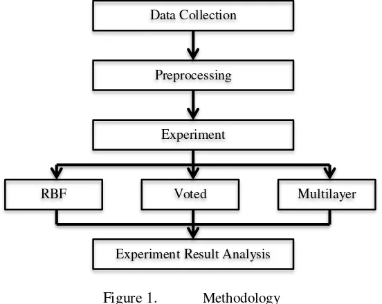
The steps compose the methodology used in this research for comparing the performance of classification algorithms is shown in Fig 1. This research was conducted in four main steps which are data collection, data preprocessing, experimentation, and result analysis. Collecting the datasets needed for conducting the experiment is the first step in the methodology. Five healthcare datasets was downloaded from UCI repository, as shown in Table I.

The next step is preprocessing. The datasets, except the Chronic Kidney Disease, are available in .txt format. There are several data formats available to present data on WEKA, include ARFF, CSV, C4.5, and XRRF. For the purpose of this research the ARFF format will be used. The other four need to be transformed into ARFF format. Using Ms. Excel the data were loaded and converted into CSV format. Then, they are converted into .arff file using WEKA.

Figure 1. Methodology Data Collection

Preprocessing

Experiment

RBF Voted

Perceptron

Multilayer Perceptron

(4)

TABLE 1. SUMMARY OF DATASET USE

Dataset Number of

Instance

Number of Attributes

Echocardiogram 106 10

SPECT Heart 267 22

Chronic Kidney Disease

450 25

Mammographic Mass 961 6

EEG Eye State 14980 6

The third step in the methodology is conducting the experiments. Three neural networks classification algorithms under test are RBF, VP, and MLP will be briefly discussed in this section.

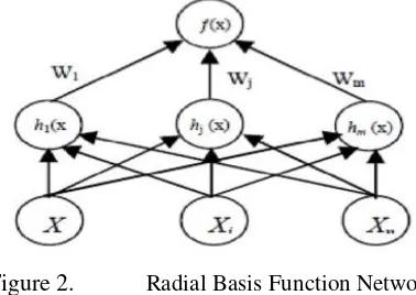
a. RBF. RBF is a feed-forward network comprised of two layers, not counting the input layer, and differs from a MLP in the way that the hidden units perform computations. Each hidden unit represents a particular point in input space, and its output for a given instance depends on the distance between its point and instance. The closer these two points, the stronger the output. RBF implements a Gaussian radial basis function network. The output layer of RBF is the same as MLP; it takes a linear combination of the outputs of the hidden units [2].

Figure 2. Radial Basis Function Network

b. Voted Perceptron (VP). VP is based on neural networks perceptron algorithm developed by Rosenblatt [15]. It works well for data that are linearly separable with large margin. The perceptron algorithm classify the data by repeatedly iterates through the training data, instance by instance, and updates the weight vector every time one the instance is misclassified based on the weights learned so far. The weight vector is updated by adding or

subtracting the instance’s attribute value to or from it. The final weigh vector is just the sum

of the misclassified instances. The perceptron makes its predictions based on whether the total weight and corresponding attribute values of instance to be classified is greater or less than zero [2].

c. Multilayer Perceptron (MLP). MLP’s architecture is characterized by the number of layers, the number of nodes in each layer, the transfer function used in each layer, and how the nodes in each layer connected to nodes in adjacent layers [15]. MLP is a feed-forward neural network based on backpropagation algorithm, with one or more hidden layers between the input and output layers. Each layer is made up of units. The inputs to the network correspond to the attributes measured for each training instance. The inputs are fed simultaneously into the units making the input layer. Then, the inputs pass through the input layer in which they

(5)

Figure 3. Multilayer Perceptron [1]

The datasets was tested using WEKA’s classifiers as shown in Table II. RBF classifier implements a normalized Gaussian radial basis function network, VP classifier implement Freund and Schapire voted perceptron algorithm, and MLP classifier uses backpropagation to classify instances [3].

TABLE 2. WEKACLASSIFIERS

Algorithms Classifier

RBF java weka.classifiers.functions.RBFNetwork

Voted

Perceptron java weka.classifiers.functions.VotedPerceptron Multilayer

Perceptron

java

weka.classifiers.function.MultilayerPerceptron

4. RESULTS AND DISCUSSION

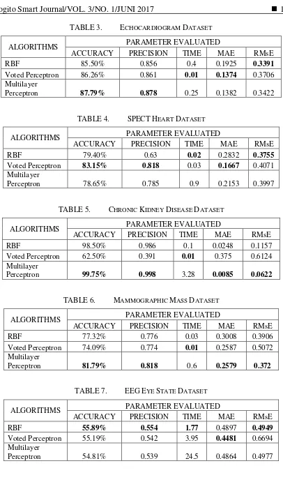
This section presents the resulting classification experiment using WEKA. Evaluation was conducted on five parameters i.e. percentage accuracy, precision, time taken to build the model, Mean Absolute Errors (MAE), and Root Means-Squared Errors (RMSE). MAE is a statistical measure to assess as to how far an estimate is from actual values, i.e., the average of the absolute magnitude of the individual errors. It is the sum over all the instances and their absolute error per instance divided by the number of instances in the test set with an actual class label [1, 2]. RMSE is a quadratic scoring rule that measures the average magnitude of the error. It is the difference between the values predicted by a model and corresponding observed values, they are each squared and the averaged over the instances. It is considered as ideal if RMSE value is small, and MAE is smaller than RMSE.

(6)

TABLE 3. ECHOCARDIOGRAM DATASET

ALGORITHMS PARAMETER EVALUATED

ACCURACY PRECISION TIME MAE RMsE

RBF 85.50% 0.856 0.4 0.1925 0.3391

Voted Perceptron 86.26% 0.861 0.01 0.1374 0.3706 Multilayer

Perceptron 87.79% 0.878 0.25 0.1382 0.3422

TABLE 4. SPECTHEART DATASET

RBF 79.40% 0.63 0.02 0.2832 0.3755

Voted Perceptron 83.15% 0.818 0.03 0.1667 0.4071 Multilayer

Perceptron 78.65% 0.785 0.9 0.2153 0.3997

TABLE 5. CHRONIC KIDNEY DISEASE DATASET

RBF 98.50% 0.986 0.1 0.0248 0.1157

Voted Perceptron 62.50% 0.391 0.01 0.375 0.6124

Multilayer

Perceptron 99.75% 0.998 3.28 0.0085 0.0622

TABLE 6. MAMMOGRAPHIC MASS DATASET

RBF 77.32% 0.776 0.03 0.3008 0.3906

Voted Perceptron 74.09% 0.774 0.01 0.2587 0.5072 Multilayer

Perceptron 81.79% 0.818 0.6 0.2579 0.372

TABLE 7. EEGEYE STATE DATASET

RBF 55.89% 0.554 1.77 0.4897 0.4949 Voted Perceptron 55.19% 0.542 3.95 0.4481 0.6694 Multilayer

(7)

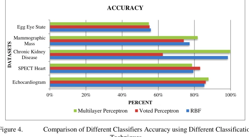
In terms of accuracy, results show that on average the MLP classifiers achieve the highest accuracy 80.56%, followed by RBF 79.32%, and VP 72.24%. MLP performs well in three datasets, echocardiogram, chronic kidney disease, and mammographic mass.

Figure 4. Comparison of Different Classifiers Accuracy using Different Classification Techniques

VP obtains the highest accuracy for SPECT Heart dataset. As for EEG Eye State dataset, all the three algorithms achieve the lowest accuracy percentage; they are less than 50%.

The experiment results also indicate that precision values represent the same type of result with accuracy. It can be seen that Fig. 3 and 4 are similar in many cases. MLP gives the highest precision values for Echocardiogram (0.878), Chronic Kidney Disease (0.998), and Mammographic Mass (0.818). VP gives the highest precision for SPECT Heart dataset (0.818). On average, the resulting classifier using MLP algorithms achieve 0.8 for precision value, followed by RBF (0.76) and VP (0.68).

(8)

TABLE 8. ERROR RATE MEASURES FOR CLASSIFICATION ALGORITHMS

Dataset RBF Voted Perceptron

Multilayer Perceptron

MAE RMsE MAE RMsE MAE RMsE

Echocardiogram 0.1925 0.3391 0.1374 0.3706 0.1382 0.3422 SPECT Heart 0.2832 0.3755 0.1667 0.4071 0.2153 0.3997 Chronic Kidney Disease 0.0248 0.1157 0.375 0.6124 0.0085 0.0622

Mammographic Mass 0.3008 0.3906 0.2587 0.5072 0.2579 0.372

EEG Eye State 0.4897 0.4949 0.4481 0.6694 0.4864 0.4977

Another parameter assessed in this research is MAE and RMSE, the error rate measures

that also determine the classifiers’ accuracy. Resulted MAE and RMSE of the algorithms tested

have met the ideal standard, in which the RMSE values are small, and the MAE values are smaller than the RMSE values. Table 8 shows the comparison of MAE and RMSE of the resulting classifiers; the best MAE and RMSE value are printed bold. VP algorithms achieve the lowest MAE in three datasets (Echocardiogram, SPECT Heart, EEG Eye State), while MLP perform better in Chronic Kidney Disease and Mammographic Mass datasets. As for RMSE,

RBF is better compare to VP. On average, MLP’s MAE and RMSE value 0.22 and 0.33, closely

followed by RBF with 0.26 and 0.34, and VP with 0.28 and 0.51.

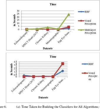
Figure 6. (a). Time Taken for Building the Classifiers for All Algorithms; (b) Time Taken for Building the Classifiers for RBF and VP

(9)

Fig. 5 (a) and (b) present the performance of three neural networks classification algorithms used in the experiment, with respect to the time taken to build the classifiers for five datasets. Fig 5(a) presents the time taken to build the classifier for all algorithms, while Fig. 5(b) shows the performance of RBF and VP distinctly since they are overlapped in Fig. 5(a). In terms of time taken for building the classifier, VP takes the lowest time for SPECT Heart and EEG Eye State datasets; RBF performs better on Echocardiogram, Chronic Kidney Disease, and Mammographic Mass datasets. On average, RBF is the fastest compare to the other two. On the other hand, MLP requires the longest time for building the classifiers.

5. CONCLUSION

Three neural networks classification algorithms performance comparison have been tested on five healthcare datasets. After the experiment and analysis of the results, the following conclusions were drawn:

1. MLP provide better classifier for most of the datasets with average accuracy of 80.56% and average precision value of 0.8. RBF shows moderate performance with average accuracy percentage of 79.32%, average precision value of 0.76. VP has the lowest average percentage of accuracy and precision value, 72.25% and 0.68 respectively.

2. For MAE results, on average, MLP’s classifier model is superior compare to the other two. 3. There is a trade-off between accuracy and classifier building time. MLP requires the longest

time (in average), 5.906 seconds, for building the classifier models. The advantage of RBF observed in this study is it spent small amount of time to build the classifier models. In terms of training time, VP algorithms’ is moderate, at 0.802 seconds. Overall, all the three

algorithms’ training time will increase as the dataset size increase.

Overall, MLP algorithm is the highest for all performance parameter tested. It can produce high accuracy classifier model but suffer in training time especially of large dataset.

REFERENCES

[1] Han J, Kamber M. Data Mining Concepts and Techniques, Academic Press: USA, 2001. [2] Witten I H, Frank E. Data Mining Practical Machine Learning Tools and Techniques. 2nd

edn. Morgan Kaufmann, 2005.

[3] WEKA. http://www.cs.waikato.ac.nz/~ml/weka. Date Accessed: 14/02/2015. [4] UCI. https://archive.ics.uci.edu/ml/datasets.html. Date Accessed: 16/02/2015.

[5] Venkatesann E, Velmurugan T. Performance Analysis of Decisin Tree Algorithms for Breast Cancer Classification. Indian Journal of Science and Technology. 2015 Nov; 8 (29).

[6] Rahman R.M, Afroz F. Comparison of Various Classification Techniques Using Different Data Mining Tools for Diabetes Diagnosis. Journal of Software Engineering and Applications. 2013; 6: 85-97.

[7] Akinola SO, Oyabugbe OJ. Accuracies and Training Time of Data Mining Clasification Algorithms: an Empirical Comparative Study. Journal of Software Engineering and Applications. 2015 Sept; 8: 470-477.

[8] Danjuma K, Osofisan A. Evaluation of Predictive Data Mining Algorithms in Erythemato-Squamous Disease Diagnosis. International Journal of Computer Science Issues. 2014; 11(6): 85-94

(10)

[10] Amin MN, Habib MA. Comparison of Different Classificaiton Techniques Using WEKA for Hematological Data. American Journal of Engineering Research. 2015; 4 (3): 55-61. [11] Durairaj, M, Deepika, R. Comparative Analysis of Classificatin Algorithms for the

Prediction of Leukimia Cancer. International Journal of Advanced Research in Computer Science and Software Engineering. 2015 Aug; 5 (8): 787-791.

[12] Barnaghi PM, Sahzabi VA, Bakar AA. A Comparative Study for Various Methods of Classification. Proc. of Int. Conf. on Informatin and Computer Networks, Singapore, 2012.

[13] Gupta N, Rawal A, Narasimhan VL, Shiwani S. Accuracy, Sensitivity and Specifity Measurement of Various Classificatin Techniques on Healthcare Data. IOSR Journal of Computer Engineering. 2013 May-June; 11 (5): 70-73.

[14] Kumar Y, Sahoo G. Analysis of Bayes, Neural Network and Tree Classifier of Classification Technique in Data Mining using WEKA. Computer Science and Information Technology. 2012; 2 (2): 359-369.

[15] Zhang, G.P. Neural Networks for Data Mining. In: Data Mining and Knowledge Discovery Handbook, 2nd_{edn., Springer, 2010; 419-444.}

[16] Nookala, G. K. M, Pottumuthu, B. K, Orsu, N, Mudunuri, S. B. Performance Analysis and Evaluation of Different Data Mining Algorithms used for Cancer Classification. International Journal of Advanced Research in Artificial Intelligence. 2013; 2(5): 49-55. [17] Mala, V, Lobiyal, D. K. Evaluation and Performance of Classification Methods for

Medical Data Sets. International Journal of Advanced Research in Computer Science and Software Engineering. 2015 Nov; 5 (11): 336-340.