Vol. 23, No. 1 (2017), pp. 27–42.
A COLLOCATION METHOD FOR SOLVING
FRACTIONAL ORDER LINEAR SYSTEM
M. Mashoof
1, A.H. Refahi Sheikhani
2∗, and H. Saberi Najafi
31Department of Applied Mathematics, Faculty of Mathematical Sciences,
Lahijan Branch, Islamic Azad University, Lahijan, Iran. [email protected]
2Department of Applied Mathematics, Faculty of Mathematical Sciences,
Lahijan Branch, Islamic Azad University, Lahijan, Iran. *Corresponding author: ah [email protected],
3Department of Applied Mathematics, Faculty of Mathematical Sciences,
Lahijan Branch, Islamic Azad University, Lahijan, Iran. [email protected]
Abstract. In the current paper we propose a collocation method to achieve an
algorithm for numerically solving of fractional order linear systems where a fractional derivative is defined in the Caputo form. We have used the Taylor collocation method for solving fractional differential equations; a collocation method which is based on taking the truncated Taylor expansions of the vector function’s solution in the fractional order linear system and substituting their matrix forms into the system. Through using collocation points we have obtained a system of linear algebraic equation. The method has been tested by some numerical examples.
Key words and Phrases: Fractional system, collocation method, numerical
simula-tion.
Abstrak. In the current paper we propose a collocation method to achieve an
algorithm for numerically solving of fractional order linear systems where a fractional derivative is defined in the Caputo form. We have used the Taylor collocation method for solving fractional differential equations; a collocation method which is based on taking the truncated Taylor expansions of the vector function’s solution in the fractional order linear system and substituting their matrix forms into the system. Through using collocation points we have obtained a system of linear algebraic equation. The method has been tested by some numerical examples.
Kata kunci: Sistem fraksional, metode kolokasi, simulasi numerik.
2000 Mathematics Subject Classification: 26A33, 74H15. Received: 15-05-2016, revised: 30-01-2017, accepted: 01-02-2017.
28
1. Introduction
Fractional differential equations have been generalized from integer order derivatives through replacing the integer order derivatives by fractional ones. The field of fractional differential equations has received attention and interest only in the past 20 years or so [2, 4, 3]. In recent years, studies concerning the application of the fractional differential equations in science has attracted more interest among scholars [9, 5]; readers can refer to [7, 8] for the theory and applications of fractional calculus in this regard. For instance, [10, 15] formulated the motion of a rigid plate immersing in a Newtonian fluid. They show that the use of fractional derivatives for the mathematical modelling of viscoelastic materials is quite natural [19]. It should be mentioned that the main reason for the theoretical development here is the wide use of polymers in various fields of engineering [19]. Moreover, in 1991, S. Westerlund in a paper on electrochemically polarizable media proposed the use of fractional derivatives for the description of propagation of plane electromagnetic waves in an isotropic and homogeneous lossy dielectric [19]. Caputo suggested the fractional order version of the relationship between the electric field and electric flux density [19].
Recently, fractional derivatives have been used to new applications in neu-ral networks and control system [5, 6, 20]. Seveneu-ral methods such as Haar-wavelet operational matrix method have exited to solve the fractional linear system [16]. In [16] the authors introduced Haar-wavelet operational matrix method for frac-tional control system and translated the control system with initial condition into
a Sylvester equation. A typical n-term linear non-homogeneous fractional order
differential equation in time domain can be described as the following form
an(Dαn
t y(t)) +· · ·+a1(Dαt1y(t)) +a0(Dtα0y(t)) =u(t). (1)
A fractional order system described byn-term fractional differential (1) can
be rewritten to the state-space representation in the form [12, 24]:
aDtβx(t) =Ax(t) +Bu(t)
y(t) =Cx(t) . (2)
For this reason, the behavior of output in system (2) is useful. Recently, the collo-cation method has become a very useful technique for solving differential equations [18, 13, 1]. In the current study, we present a numerical solution of the fractional order system through the use of Taylor collocation method for a system of the form
aDαtx(t) =Ax(t) +Bu(t)
y(t) =Cx(t) +Du(t),
0≤t≤η, x(0) = λ1, λ2,· · · , λn
T ,
(3)
with 0< α≤1, whereA,B,CandDaren×n,n×m,p×nandp×mmatrices,
andu(t) is anm-vector function, andaDαtx(t) is theαth-order (always fractional)
derivative ofx(t) in the Caputo form. By using this method, we can translate (3)
This paper is organized as follows. We review some basic definitions of frac-tional derivative operators. The function approximations and two applicable algo-rithms are presented in section 3. Section 4 contains four examples, and finally, conclusions are presented in section 5.
2. Basic Definition and Theorem
Here and in this part of the study, we deal with fractional calculus, definitions and theorems; see [23, 14, 17]. for more details in this regard.
Definition 2.1. A real function f(x), x ≥ 0 is said to be in space Cµ, µ ∈ R if
there exists a real number p(> µ), such thatf(x) =xpf
1(x)where f1(x)∈[0,∞),
and it is said to be in the space Cm
µ ifffm∈Cµ, m∈N.
Definition 2.2. The Riemann-Liouville fractional derivative of order α with
re-spect to the variablexand with the starting point atx=ais
aDαtf(x) =
Definition 2.3. The Riemann-Liouville fractional integral of orderαis
aD
Definition 2.4. The fractional derivative off(x)in the Caputo form is defined as
Dαtf(x) = 1
For the Caputo’s derivative we haveDα
tC= 0, andCis a constant. Moreover,
is a vector function, we define
30
Now consider the fractional differential equations as
Dα
tx(t) =Ax(t) +q(t), (9)
where 0 < α < 1, A is an N ×N matrix, and q : [0, h] → CN. Two following
theorems show the form of the general solution of (9) whereEα(t) is the
Mittag-Leffler function.
Definition 2.6. The Mittag-Leffler function with parameterαis given by
Eα(z) =
the corresponding eigenvectors; then the general solution of the homogeneous
dif-ferential equationDαtx(t) =Ax(t)will be
x(t) = N X
l=1
clu(l)Eα(λlxα), (10)
with certain constants cl ∈ C. The unique solution of this differential equation
subject to the initial conditionx(0) =x0 is characterized by the linear system
x0= (u(1),· · ·, u(N))(c1,· · ·, cN)T. (11)
Proof. See [11].
For the inhomogeneous boundary value problem, we have the following the-orem.
Theorem 2.8. The general solution of the boundary value problem (9) has the form
x=xhom+xinhomwherexhom is the general solution of the associated homogeneous
problem andxinhom is a particular solution of the inhomogeneous problem.
Proof. See [11].
Following we recall the generalization of Taylor formula which forms the basis of our numerical method.
Theorem 2.9. (generalized Taylor formula) Suppose that Dkα
We can use the generalized Taylor formula in the matrix form as follows
hence we can approximatef(x) as follows
f(x)≃X(x)M0v. (17)
Moreover, we have
32
3. Numerical method
In this section, we present two algorithms for numerical solution of system (3) based on Taylor collocation method. For this, we use equations (14) and (19)
for each array of vector functionx(t), and it’s fractional derivative, namely as
xj(t)≃xNj =X(t)M0vj, (22)
and
Dtαxj(t)≃DtαxjN(t) =X(t)M1M0vj. (23)
If we use (22) and (23) to approximatexj(t) andDα
txj(t)f or j= 1,· · ·n; then we
have a system of linear equations.
Theorem 3.1. If we approximatexj(t)andDtαxj(t)forj = 1,· · ·n, by (22) and
(23) respectively; then we have a system of linear equations as XeFeev =eb where
e
v= (v, v,· · ·, v)T.
Proof. By substituting equations (22) and (23) in equation (3) we have
v=
Dispersing equation (24) by the collocation points ti, i= 0,1, ..., N, we can
obtain
X(ti)F v=β(ti),
where
F = (A∗I−M1)M0. (28)
Now we find the matrix representation of the initial conditionx(a),
X(a)M0vj =λj f or j = 1,2, ..., n , (29)
To obtain the numerical solution of (3), by replacingX(tN)F v=β(tN) with
equa-tion (29), we have the new algebraic equaequa-tion,
or in blocked matrix form
34
hence we obtain a system ofn(N+ 1)2 linear algebraic equations withn(N+ 1)2
unknown Taylor coefficients for xi(t), i= 1,2, ..., n.
From above discussions we find that
vi= y(i−1)(N+1)+1 y(i−1)(N+1)+2 · · · y(i−1)(N+1)+N yi(N+1) , (35)
which is the vector of Taylor coefficients forxi(t), i= 1,2, ..., n.
The algorithm is
Ifa≤t≤band (b−a) are large, we can divideI= [a, b] intoI1= [a, t1], I2=
[t1, t2],· · ·, IN = [tN−1, b] and approximatex(t) on subinterval Ik+1 and use the
approximated solution attk+1to initial condition of next subinterval. The following
Lemma shows that by this procedure error can be decreased.
Lemma 3.3. Letx(t)be bounded on[a, b]. If we useI1= [a, t1], I2= [t1, t2],· · · , IN =
[tN−1, b]and approximatex(t)on subintervalIk+1and use approximated solution at
tk+1 to initial condition of next subinterval, absolute error at time t=b decreases.
Proof. From (12), for intervalI, if|DtN+1xi(ζ)|< li; then we have
e=|xi(b)−xNi (b)|
=|DNt +1xi(ζ)| (b−a)(N+1)α
Γ((N+1)α+1) < li (b
−a)(N+1)α Γ((N+1)α+1)
=Li(N h)(N+1)α,
(36)
whereh= b−a
N . Moreover, for subintervalIj we have
ej=|xi(tj)−xNi (tj)|< li(tj−tj−1)
(N+1)α
Γ((N+ 1)α+ 1) =Lih
(N+1)α;
thus
e1+e2+· · ·+eN < LiN h(N+1)α< Li(N h)(N+1)α=e.
This shows that the following algorithm can be more efficient than algorithm
3.2 att=b.
Proposition 3.4. InputA, B, x(a), u(t), N, a, b
Outputx(b)
1.fori= 0,1,· · · , N−1 do
Set Ii= [ti, ti+ 1], a=ti, b=ti+1
Utilize algorithm 3.2 and approximatex(ti+1)
Set x(a) =x(ti+1)
2. Set x(b) =x(tN)
end do.
4. Numerical Examples
36
fractional linear systems whose exact solutions are known. We usek.k2to compare
the exact and numerical solutions.
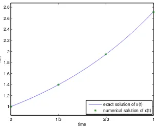
Example 4.1. Let us consider the following system with the initial conditions
Dαtx(t) =
We approximately solve the above system for N = 10and obtain the approximate
solution for α= 1 as
In figure 1 we can see the numerical and exact solutions.
Example 4.2. Let us consider following fractional equation
Dαtx(t) =x(t);x(0) = 1; 0≤t≤1; (39)
the exact solution, when α= 1, is
x(t) =et, (40)
and forα=12 is
x(t) =et(erf√t+ 1). (41)
We approximately solve fractional equation (39) forα= 1withN = 3and obtained
the approximate solution,
0 1/10 2/10 3/10 4/10 5/10 6/10 7/10 8/10 9/10 1
exact solution of x1(t) exact solution of x
2(t) numerical solution of x1(t) numerical solution of x2(t)
Figure 1. Numerical and exact solution of example 4.1 forα= 1
andN = 10.
exact solution of x(t) numerical solution of x(t)
Figure 2. Numerical and exact solution of example 4.2 forα= 1
andN = 3.
In figure 2 we can see the numerical and exact solutions of example 4.2 for
α= 1 with N = 3; Moreover, figure 3 shows the results forα= 0.5 withN = 9 in
example 4.2.
38
exact solution of x(t) numerical solution of x(t)
Figure 3. Numerical and exact solution of example 4.2 for α=
0.5 andN = 9.
exact solution of x 1(t)
exact solution of x2(t)
exact solution of x3(t)
numerical solution of x1(t)
numerical solution of x2(t)
numerical solution of x3(t)
Figure 4. Numerical and exact solution of example 4.3 for α=
0.975 andN = 5.
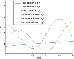
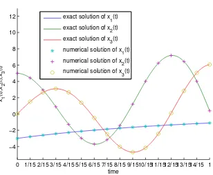
The general solution of this system according to theorems 2.7 and 2.8 is given by
x(t) =c1u1Eα(λ1tα) +c2u2Eα(λ2tα) +c3u3Eα(λ3tα), (43)
wherec1, c2, c3 are constants, λ1, λ2, λ3 are eigenvalues, andu1, u2, u3 are the
cor-responding eigenvectors of A.
In the figures 4 and 5 the numerical and exact solutions of x(t)forα= 0.975 are
shown for N = 5 and N = 15, respectively. From figure 4 we can see that the
numerical solution withN = 5is not a mismatch with the exact solution, but from
figure 5 we can see that the numerical solution is in very good agreement with the
exact solution forN= 15. Moreover, the errors of numerical solutions for different
N are shown in table 1. From table 1 we can see that the numerical solutions are
more and more close to the exact solution when the value ofN becomes large.
Example 4.4. Consider example 4.3 with t ∈ [0,3], N = 16 and divide [0,3] to
0 1/15 2/15 3/15 4/15 5/15 6/15 7/15 8/15 9/1510/1511/1512/1513/1514/15 1
exact solution of x 1(t) exact solution of x2(t) exact solution of x3(t) numerical solution of x1(t) numerical solution of x2(t) numerical solution of x3(t)
Figure 5. Numerical and exact solution of example 4.3 for α=
0.975 andN = 15.
Table 1. Error of approximated solution in example 4.3
N error at t=1
4 1.0966 1.6726 2.2574
8 0.0352 0.0366 0.0488
16 1.5671e-07 4.4075e-07 0.0016
32 4.1904e-12 3.8083e-07 0.0016
Table 2. Error of approximated solution in example 4.4 at t=b
by algorithm 3.2 and algorithm 3.4.
subinterval [0,1] [1,2] [2,3] [0,3]
algorithm 3.2 3.2 3.2 3.4
error at time b 9.1359e-07 6.7420e-05 0.0014 690.6396
compare the results. The numerical results will presented in table 2. From table 2
we see that if we use algorithm 3.2, the error at time t = 3 is 690.6396 which is
unacceptable, but with dividing interval [0,3] into three intervals [0,1],[1,2],[2,3]
and use algorithm 3.4, the error at timet= 1,2and3is9.1359e−07,6.7420e−05
and 0.0014, respectively. This example confirms Lemma 3.2, and so we see that
algorithm 3.4 is useful.
In figure 6 we can see the numerical and exact solutions of example 4.4 with
N = 16 by algorithm 3.2. Figures 7, 8, and 9 show the numerical and exact
40
exact solution of x
1(t)
exact solution of x2(t)
exact solution of x
3(t)
numerical solution of x1(t)
numerical solution of x
2(t)
numerical solution of x
3(t)
Figure 6. Numerical and exact solution of example 4.4 on [0,3]
by algorithm 3.2.
0 0.2 0.4 0.6 0.8 1
exact solution of x
1(t)
exact solution of x2(t)
exact solution of x3(t)
numerical solution of x1(t)
numerical solution of x2(t)
numerical solution of x3(t)
Figure 7. Numerical and exact solution of example 4.4 on [0,1]
by algorithm 3.4.
5. Conclusions
1 1.2 1.4 1.6 1.8 2
numerical solution of x1(t)
numerical solution of x
2(t)
numerical solution of x3(t)
Figure 8. Numerical and exact solution of example 4.4 on [1,2]
by algorithm 3.4.
2 2.2 2.4 2.6 2.8 3
numerical solution of x1(t)
numerical solution of x2(t)
numerical solution of x3(t)
Figure 9. Numerical and exact solution of example 4.4 on [2,3]
by algorithm 3.4.
results show that this method is extremely effective and practical for this sort of approximate solutions. This method will be applicable in large domains as well.
References
[1] Aminikhah, H., Refahi Sheikhani, A. and Rezazadeh, H., ”Travelling wave solutions of non-linear systems of PDEs by using the functional variable method”,Bol. Soc. Paran. Mat.,34 (2016), 213-229.
[2] Aminikhah, H., Refahi Sheikhani, A. H. and Rezazadeh, H., ”Sub-equation method for the fractional regularized long-wave equations with conformable fractional derivatives”,Scientia
Iranica,23(2016), 1048-1054.
[3] Aminikhah, H., Refahi Sheikhani, A. H. and Rezazadeh, H., ”Exact solutions of some non-linear systems of partial differential equations by using the functional variable method”,
42
[4] Aminikhah, H., Refahi Sheikhani, A. H. and Rezazadeh, H., ”Approximate analytical solu-tions of distributed order fractional Riccati differential equation”,Ain Shams Engineering
Journal, Article in press.
[5] Aminikhah, H, Refahi Sheikhani, A. and Rezazadeh, H., ”Stability Analysis of Distributed Order Fractional Chen System”,The Scientific World Journal,2013(2013), 1-13.
[6] Aminikhah, H, Refahi Sheikhani, A. and Rezazadeh, H., ”Stability analysis of linear dis-tributed order system with multiple time delays”,U.P.B. Sci. Bull.,77(2015), 207-218. [7] Ansari, A. and Refahi Sheikhani, A., ”New identities for the Wright and the Mittag-Leffler
functions using the Laplace transform”,Asian-European Journal of Mathematics,7(2014), 1-8.
[8] Ansari, A., Refahi Sheikhani, A. and Kordrostami, S., ”On the generating functionext+yφ(t) and its fractional calculus”,Cent. Eur. J. Phys.,11(2013), 1457-1462.
[9] Ansari, A., Refahi Sheikhani, A. and Saberi Najafi, H., ”Solution to system of partial frac-tional differential equations using the fracfrac-tional exponential operators”, Math. Meth. Appl. Sci.,35(2012), 119-123.
[10] Das, S., ”Functional Fractional Calculus, 2nd Edition”,Springer-Verlag, Berlin, Heldelberg, (2011).
[11] Diethelm, K., ”The Analysis of Fractional Differential Equations: An Application-Oriented Exposition Using Differential Operators of Caputo Type”, vol. 2004 of Lecture Notes in
Mathematics, Springer, Berlin, Germany, (2010).
[12] Dorcak, L., Petras, I., Kostial, I. and Terpak, J., ”Fractional-order state space models”,Proc.
of the International Carpathian Control ConferenceICCC2002, Malenovice, Czech republic,
May 27-30, 193-198.
[13] Gulsu, M. and Sezer, M., ”A Taylor polynomial approach for solving differential-difference equations”,Journal of Computational and Applied Mathematics,186(2006), 349-364. [14] Karamete, A. and Sezer, M., ”A Taylor collocation method for the solution of linear
integro-differential equations”, International Journal of Computer Mathematics, 79 (2002), 987-1000.
[15] Luo., A.C.J., ”Dynamical Systems: Discontinuity, Stochasticity and Time-Delay”,Springer, (2010).
[16] Mashoof, M. and Sheikhani, A. H. R., ”Numerical solution of fractional control system by Haarwavelet operational matrix method”,Int. J. Industrial Mathematics,8(2016), 289-298. [17] Odibat, Z. M. and Shawagfeh, N. T., ”Generalized Taylors formula”,Applied Mathematics
and Computation,186(2007), 286-293.
[18] Ozturk, Y., AnapalJ, A., Gulsu, M. and Sezer, M., ”A Collocation Method for Solving Fractional Riccati Differential Equation”,Journal of Applied Mathematics,2013(2013), 1-8. [19] Podlubny, I., ”Fractional differential equations”,Mathematics in Science and Engineering,
Academic Press, New York, NY, USA.,198(1999)
[20] Rezazadeh, H., Aminikhah, H. and Refahi Sheikhani, A., ”Stability analysis of Hilfer frac-tional differential systems”,Math. Commun.,21(2016), 45-64.
[21] Saberi Najafi, H., Edalatpanah, S., A. and Refahi sheikhani, A. H., ”Convergence Analysis of Modified Iterative Methods to Solve Linear Systems”,Mediterranean Journal of
Mathe-matics,11(2014), 1019-1032.
[22] Saberi Najafi, H. and Refahi, A., ”A new restarting method in the Lanczos algorithm for generalized eigenvalue problem”,Applied Mathematics and Computation,184(2007), 421-428.
[23] Sezer, M., ”Taylor polynomial solutions of Volterra integral equations”,International Journal
of Mathematical Education in Science and Technology,25(1994), 625-633.
[24] Yang, C. and Liu, F., ”A computationally efective predictor-corrector method for simulat-ing fractional order dynamical control system”,Australian and New Zealand Industrial and
![Figure 6. Numerical and exact solution of example 4.4 on [0, 3]by algorithm 3.2.](https://thumb-ap.123doks.com/thumbv2/123dok/962988.844256/14.595.219.375.343.463/figure-numerical-exact-solution-example-algorithm.webp)
![Figure 8. Numerical and exact solution of example 4.4 on [1, 2]by algorithm 3.4.](https://thumb-ap.123doks.com/thumbv2/123dok/962988.844256/15.595.215.373.309.430/figure-numerical-exact-solution-example-algorithm.webp)
