getdocf99b. 551KB Jun 04 2011 12:05:14 AM

(1)

E l e c t ro n ic

Jo u r n

a l o

f P

r o b

a b i l i t y

Vol. 7 (2002) Paper No. 13, pages 1–74. Journal URL

http://www.math.washington.edu/~ejpecp/ Paper URL

http://www.math.washington.edu/~ejpecp/EjpVol7/paper13.abs.html

MULTIPLE SCALE ANALYSIS OF SPATIAL BRANCHING PROCESSES UNDER THE PALM DISTRIBUTION

Anita Winter

Mathematisches Institut, Universit¨at Erlangen-N¨urnberg Bismarckstraße 1 1/2, 91054 Erlangen, Germany

winter@mi.uni-erlangen.de

Abstract We consider two types of measure-valued branching processes on the latticeZ

d_{. These} are on the one hand side a particle system, called branching random walk, and on the other hand its continuous mass analogue, a system of interacting diffusions also called super random walk. It is known that the long-term behavior differs sharply in low and high dimensions: if d ≤ 2 one gets local extinction, while, for d_≥ 3, the systems tend to a non-trivial equilibrium. Due to Kallenberg’s criterion, local extinction goes along with clumping around a ’typical surviving particle.’ This phenomenon is called clustering.

A detailed description of the clusters has been given for the corresponding processes on R

2 _in

[28]. Klenke proved that with the right scaling the mean number of particles over certain blocks are asymptotically jointly distributed like marginals of a system of coupled Feller diffusions, called system of tree indexed Feller diffusions, provided that the initial intensity is appropriately increased to counteract the local extinction. The present paper takes different remedy against the local extinction allowing also for state-dependent branching mechanisms. Instead of increasing the initial intensity, the systems are described under the Palm distribution. It will turn out together with the results in [28] that the change to the Palm measure and the multiple scale analysis commute, ast_{→ ∞}.

(2)

(3)

1 Introduction

In this paper we consider interacting branching models on the latticeZ

d_{, where the interaction is} due to migration between the sites ofZ

d_{, and hence, linear. Their basic ergodic theory is the same} as that of a wide class of interacting processes with components indexed byZ

d_{, by}

R

d_{, or by the} hierarchical group. On the one hand, this class includes interacting particle models, for example the voter model (Holley and Liggett (1975) [23]), branching random walk (Kallenberg (1977) [25], Durrett (1979) [14]), or branching Brownian motion (Fleischman (1978) [19], Gorostiza and Wakolbinger (1991) [22]), and on the other hand, interacting diffusions, for instance the Fisher– Wright stepping stone model (Shiga (1980) [36]), the Ornstein–Uhlenbeck process (Deuschel (1988) [13]), or super Brownian motion (Dawson (1977) [7], Etheridge (1993) [17]). For all these processes the long term behavior depends on whether the underlying migration is recurrent or transient; hence it differs sharply in high and low dimensions. In high dimensions each process has a one-parameter family of invariant measures indexed by the ’intensity’ of the system which is preserved. In low dimensions the invariant measures are ’degenerate’, that is, steady states are concentrated on traps - the systems cluster. For branching models this means that mass becomes locally extinct while the surviving mass piles up at spatially rare sites.

For many models the structure of the clusters is well-studied. These models are e.g. the voter model inZ

d_,_d_{= 1,}_{2, (Cox and Griffeath (1986) [6]), linearly interacting diffusions with compact} state space indexed by the hierarchical group (Dawson and Greven (1993) [9], [10], Fleischmann and Greven (1994) [20], Dawson, Greven and Vaillancourt (1995) [12], Klenke (1996) [27]) and interacting Brownian motions indexed byZ

d_,_d_{= 1,}_{2, (Kopietz (1998) [31], Klenke (2000) [30]).} The concepts of describing phenomena concerning clustering includerenormalization,averaging and rescaling.

The present paper describes the cluster formation of the branching models in the critical di-mension,dc = 2. It has turned out that the growth rate of a cluster is determined by theGreen function of the migration kernel. In two dimensions the Green function grows very slowly, namely on a logarithmic scale. This implies the phenomenon ofdiffusive clusteringwhich means that the clusters extend in space astα2, where α∈[0,1) is a random order.

Clusters of branching models in the diffusive regime are investigated in [19], [14], Lee (1991) [32], Dawson and Greven (1996) [11], and Klenke (1997) [28], (1998) [29]. While the first three papers mentioned attempt to describe the rate of growth of clusters, the latter three give an insight into the spatial profile by considering space-time respectively space renormalized systems. The main points of our paper are twofold. First, in comparison with [28], in addition to the spatial structure, we formulate and prove more detailed statements about how clusters evolve in time and about the family structures in a cluster. Secondly, we exhibit how the clustering phenomena can be studied by zooming into a cluster in a way which allows also for state-dependent branching mechanisms. In the context of models with the branching property that means to use techniques from the theory of infinitely divisible systems. We describe now these two points.

First_{, to follow the concept of} _{multiple space-time scaling, we have to rescale the space-time} correlation structure among n components situated at sites yi

(5)

cover the multiple-scale situation. Our aim will be to show that due to the diffusive clustering regime the correlation structure reduces to the knowledge of the two by two space-time distances di,j_t :=_|si_t₋sj_t_{| ∨ k}y_ti₋y_tj _k2_≈t1−Ai,j, (1.1) whereAi,j denotes thefunction of scaling exponents. In order to describe with these exponents the diffusive clustering we construct a process which we call a system of tree indexed Feller diffusions. Since branching is naturally connected with genealogical trees or more generally with genealogical groves, we introduce the grove indexed systems which are lurking in the back. In the theory of measure-valued processes a treatment using a multiple scale analysis via tree indexed diffusions can be found in the following situations: for a compact state space model in Fleischmann and Greven (1996) [20], for Gaussian fields which allow an explicit calculation in [31], and for super Brownian motion in [28], [29].

Secondly_{, branching systems, which have components in [0,}_∞_{), become extinct. This means} that ’clusters at _∞’ have a probability going to 0. In contrast to processes with components in [0,1] ([20]) or in (_−∞,_∞) ([31]), for processes with components in [0,_∞) it is not possible to find a suitable renormalization such that the renormalized components tend to a non-trivial limit. Hence, we additionally need a trick to be able to observe a cluster.

An obvious way to focus on clusters is tocondition the branching model on local non-extinction. This approach has been chosen by Lee (1991) [32] for the corresponding particle system on R

2_,

and Dawson and Greven (1996) [11] for interacting diffusions (containing the case of branching diffusions) with components indexed by the hierarchical group. Unfortunately, none of the techniques used in [32] and [11] work out for the lattice. It is not even understood what here the suitable condition for local non-extinction is.

A way out of conditioning is to blow up the initial intensity to ensure that one finds surviving mass in a particular window in space. This is first done by Klenke ([28], [29]) for branching models on R

2_{, and can be extended to the lattice. But by blowing up we observe a random}

number of families in every bounded set, and we hence loose a slight amount of information on the family structure. Moreover, the method would fail in models with state-dependent branching. We therefore choose an other approach: instead of concentrating on a ’typical site with surviving mass’, we rather describe the space-time picture from the perspective of a ’typical surviving member of the population’. In translation invariant and shift ergodic situations that means rescaling the systems under thePalm distribution. It will turn out that under the Palm measure we are in a position to focus on a single family.

The main emphasis of this paper will, consequently, be to use the concept of size-biasing, and make then use of the explicit calculations by exploiting the branching property. We consider simultaneously branching particle systems and their continuous mass analogies. In particular we rely on rescaling the closed moment hierarchy for superprocesses.

1.1 The models

(6)

1.1.1 Basic definitions

Let (E,_B(E)) be a locally compact polish space equipped with the Borel σ-algebra.

(i) A measureλon_B(E) is called(locally) finite, ifλ(B)<_∞for all (compact) setsB _{∈ B}(E). (ii) We writeMf(E) (M(E)) for the class of all these measures onB(E), and Nf(E) (N(E)) for its integer (integer or infinity) valued subclass. Forλ_{∈ M}f(E) (Nf(E)), let k λk:= λ(E).

(iii) We denote byM(E) (M+(E),M0(E)) the class of measurable functions on E (which are

non-negative, of compact support), and byC0(E) the class of continuous functionsE→R

which have compact support.

(iv) _M(E) is equipped with the vague topology generated by the maps λ _{7→ h}λ, f_i :=

R

f(x)λ(dx), f ∈ C0(E). The convergence in M(E) is denoted by −→vag. Notice that

(M(E),−→vag) is a polish space (see e.g. Kallenberg (1983) [26]).

(v) Let _M1(M(E)) (M1(Mf(E))) denote the space of all probability distributions on

B(M(E)) (B(Mf(E))). ThenM1(M(E)) (M1(Mf(E))) equipped with the weak topol-ogy is again polish. We write _⇒for the convergence of probability measures.

(vi) A(finite) random measure Φ onE is given by its distribution law,L[Φ], i.e. a probability measure P_{∈ M}1(M(E)) (P∈ M1(Mf(E))). Itsintensity measure is defined by

ΛP(B) :=E[Φ(B)], B∈ B(E). (1.2)

(vii) APoisson random field_H(µ) with locally finite intensity measure Λ_H₍_µ₎=µ_{∈ M}(E) is a random measure whose law is given by its Laplace functional: for f _∈M₀+(E) bounded,

E[exp−hH(µ), fi] = exp[−hµ, 1−e−fi]. (1.3) We denote its distribution by _POISµ.

1.1.2 Branching random walk

The basic ingredient for our processes is a time homogeneous random walk ξ = (ξt)t≥0, which

we introduce as follows: let (ξn)n∈N be a random walk in discrete-time on Z

d_{with the transition} kernel a(x, y) :=P[ξ1=y|ξ0=x]. The transition probability of its continuous time version ξ

is then given by poissonizing, i.e,

at(x, y) :=

X

n≥0

a(n)(x, y)t n_e−t

n! , (1.4)

where a(n)(·,·) denotes the n-step transition probability. We make the following assumptions on the discrete time kernela(·,·):

(7)

(ii) The kernel a(·,·) has finite second moments,

X

x∈Zd

a(0, x)kxk2<∞, (1.5)

wherek·kis the maximum norm.

(iii) Thecovariance matrix of the one-dimensional marginals Q:=E[ξ₁iξ₁j]

i,j∈{1,···,d} (1.6) with respect to the distribution

P(ξ₁1,_{· · ·} , ξ₁d) =x=a(0, x), x_∈Z

d_, _(1.7)

is assumed to be invertible, i.e., detQ₆= 0. Hence, the matrix a(·,·) is irreducible. In the following, the random walk ξ is referred to as thebasic process.

We now define the Branching Random Walk on Z

d _{with the lifetime parameter} _V _{(BRW) by} the following procedure:

Migration: Each particle starting from x_∈Z

d_{moves according to the law of} _ξ.

Branching: After a mean 1/V exponential life time the particle either dies or is replaced by 2 new particles. Each case occurs with probability 1/2.

Both mechanisms occur independently for all particles, independently of each other and inde-pendently of the initial configuration. In particular, the branching is critical in the sense that E[K] = 1, where K is the random number of new particles. The offspring behave as K inde-pendent copies of the one particle system started from the parent particle’s final site. In this way, the initial particle generates a random population at time t > 0, described by an atomic random measureηt∈ Nf(Z

d_).

We denote by (_Ss,t)t≥s the transition kernels of ξ, which describes the expected position at timetif we start in some site, say x, at time s. That is,

Ss,t[f](x) :=Eδx,s[f(ξt)], (1.8) f ∈ Cb,0(Z

d_{). We use the abbreviation} _S

t := S0,t, which defines asemigroup. Notice that due to (1.4) the generator ∆RW of (St)t≥0 on Cb,0(Z

d_{) is given by}

∆RWf = d dtSt[f]

t=0 =

X

y∈Z d

(8)

1.1.3 Super random walk

The second class of models we look at occurs as diffusion limit of the particle model previously discussed or may, alternatively, be introduced as a system of interacting diffusions constructed via SDE’. We now give both constructions.

First we consider the short life time – high intensity limit of our particle system BRW. The appropriate scaling is the following: consider a sequence (ηN)N≥1, where ηN is such that each

particle has mass _N1, the life time parameter is N V, and the initial population µN ∈ Nf(Z

d_{) is} chosen such that_N1µN

vag

→ µ, asN _{→ ∞}, for someµ_{∈ M}f(Z

d_{). Then the process}_ηN _{:= (η}N t )t≥0

converges, as N → ∞, in law to the Super Random Walk on Z

d _{with life time parameter} _V (SRW), i.e. to a Markov processX := (Xt)t≥0 with values inMf(Z

d_{) and with}_L_[X

0] =δµ (see Dawson (1993), Section 4.4 [8]).

So far, SRW is defined for finite initial configurations,µ_{∈ M}f(Z

d_{). In principle we can extend} this definition by superposing independently single ancestor processes. However, to get a decent Markov process, we want to extend the state space to a Borel space E _{⊂ M}(Z

d_{) such that} _E is invariant under the dynamic. To introduceE, we impose a regularity condition on the initial measureµ. We assume that µ∈lγp, for some p≥1, wherelpγ is constructed as follows: choose a positive and summable sequence_{γx; x∈Z

d_} _{such that for some finite constant Γ}_>_1,

X

x∈Z d

γxa(x, y)≤Γγy ∀y∈Z

d_. _(1.10)

For instance,

γx :=

X

n≥0

Γ−n X y∈Zd

a(n)(x, y)βy (1.11)

with a positive and summable sequence{βx; x∈Z

d_}_{. Then we set} lp_γ:={µ∈ M(Z

d_{) :} X x∈Zd

γxµ({x})p <∞ }. (1.12)

For L[X0] = δµ ∈ lγp we define X as the increasing limit of (Xn)n≥1 with finite initial states

µn↑µ, as n→ ∞. It then turns out that for anyt >0,Xt acquires values in lpγ ⊂ M(Z

d_{) a.s.} The same construction guarantees thatηt∈lpγ⊂ N(Z

d_{) for any} _{t >}_{0 a.s. iff} _η

0 ∈lpγ. The state space lpγ was first introduced in the context of particle systems by Liggett and Spitzer (1981) [33].

Due to the construction, the law of SRW isinfinitely divisible, a fact which justifies to callX a superprocess. To obtain an infinitely divisible law also for the particle model, choose the initial configuration Φ =Pδxk random with a Poisson distribution (compare with (1.3)).

We now come to the second description of the system given by the SRW dynamic. For µ∈l1_γ, the infinite system

χ(t) :=_{χx(t) :=Xt({x}); x∈Z

d_} _(1.13)

(9)

dχx(t) =

X

y∈Z d

[a(x, y)₋δ(x, y)]χy(t)dt+

p

g(χx(t))dwx(t), x∈Z

d_,

x(0) =µ.

Here the diffusion coefficient is g(x) :=V x, and {wx(t); x∈Z

d_}_{is a collection of independent} Brownian motions on the real line.

We know from Shiga (1992) [37] that IFD is strongly Markovian, and its infinitesimal generator Gis given by

Gf = X x∈Zd



X

y∈Zd

[a(x, y)−δ(x, y)]χy



 ∂f

∂χx + V

2

X

x∈Zd

χx ∂2f ∂χ2

x

, (1.14)

forf ∈C₀2(l1_γ), and with this generator G, in a third approach, the IFD can be constructed via semigroups.

IFD is a special case of the interacting diffusions considered in Cox, Greven, and Shiga (1994) [5], and in Cox, Fleischmann and Greven (1994) [3].

1.1.4 Analytical connection between BRW and SRW

Both classes of models just defined are connected in the sense that their laws are ruled by the same dual process, which is deterministic and given by a countable system of ODE. This system describes the Laplace transforms of ηt and Xt. It is, therefore, the discrete space analogue of the PDE known from Branching Brownian Motion (BBM) and Super Brownian Motion (SBM) on R

d_{, respectively.} _{Namely, for test functions}_f _∈_M+ 0 (Z

d_{), and} _s_≥_{0, let} _t _7→ _us

·(t;f)∈l

1

γ be non-negative solutions of thereaction diffusion equation

d dtu

s_(t;_f_{) = ∆}

RWus(t;f)− V

2(u

s_(t;_f₎₎2 _(1.15)

with the initial condition

us_·(s;f) =f. (1.16)

Unlike for SBM onR

d_{, where in the reaction diffusion equation the generator ∆}

RW is replaced by the one-half Laplacian operator, 1₂∆, on the lattice no explicit sub- or super-solutions for (1.15) in terms of a general kernel a(i, j), can be constructed. A simple renewal argument for BRW and the construction of SRW as short life-time–high-density limit show that for f _∈ M₀+(Z

d₎ solutions of (1.15) are given by

Eδx,s_[exp_−h_η

t, fi] = 1−usx(t; 1−e−f) Eδx,s_[exp_−h_X

t, fi] = exp[−usx(t;f)].

(1.17)

For this reason, (1.15) is often referred to as log-Laplace equationof the process X. Applying (1.9), (1.15) can be rewritten as integral equation

us(t;f) + V 2

Z t

s St

(10)

Recall that, for each m∈ M(Z

d_),_η _{started with} _POIS

m and X started withδm areinfinitely divisible (without any deterministic or normal contributions), i.e., there exist uniquely deter-mined measures QBRW

t := QBRW,mt on N(Z

d_{) and} _QSRW

t :=QSRW,mt on M(Z

d_{), respectively,} called thecanonical measures, such that

EPOISm_[exp_−h_η

t, fi] = exp[−

Z

N(Zd₎

(1₋ehµ,fi)QBRW_t [dµ]]

Em[exp−hXt, fi] = exp[−

Z

M(Z d₎

(1−ehµ,fe i)QSRW_t [dµ]].e

(1.19)

Observe that by the branching property we have a desintegration formula, i.e., Q·RW,m

t [dµ] =hm, Q·tRW[·,dµ]i, (1.20) whereQ·RW

t denotes the canonical measure of either ηt orXt. Recall that since a particle is non-divisible,

QBRW_t [x,·] =Pδx_[η

t∈·]. (1.21)

Moreover, we derive from (1.17) that the particle model is embedded in the continuous mass model via Poissonizing, i.e., in terms of canonical measures the following holds:

QBRW_t [·,dµ] =

Z

M(Zd₎POISµe

[dµ]QSRW_t [·,dµ]._e (1.22)

1.2 Basic ergodic theory

If we start the branching processes in a finite measure it is easy to see that the total mass tends to 0. However, as described in (1.10) to (1.12), we have used these finite mass processes to construct processes started from certain infinite measures. The question of the long-time behavior is then a more interesting one because it depends on the relative strength of the two competing mechanisms: branching and spatial migration. In low dimensions branching dominates while in higher dimensions the migration does. This dichotomy goes back to two papers which have become ’classics’: Dawson (1977) [7] dealing with SBM, and Kallenberg (1977) [25] dealing with a time-discrete branching particle model. Both papers yield the same result which can be stated as a ’metatheorem’: a recurrent particle/mass (symmetrized) migration goes along with local extinction while a (symmetrized) transient migration allows the construction of a non-trivial equilibrium with finite mass. However, the techniques used in these papers are quite different: the first one uses analytic and the second probabilistic techniques.

(11)

of second order terms. While in the recurrent case Dawson used the precise knowledge of the transition density of BM, Etheridge’s estimates lead to a proof of local-extinction also for SRW. Kallenberg’s main criterion is that local extinction appears iff the locally size-biased population in a bounded set (or in a lattice site) converges to infinity almost surely as time tends to infinity, i.e., local extinction goes along with clumping around a ’typical surviving particle’. Moreover, he presents the method of backward trees which describe the genealogy of a randomly sampled particle of generation n, and which allows the Palm distribution of the n-th generation to be computed. In Gorostiza and Wakolbinger (1991) [22] this method is extended to a class of continuous-time branching particle models containing BBM on R

d_{. This again extends to a} proof for BRW.

A direct approach to BRW can be found in Durrett (1979) [14]. The proofs of Durrett’s results are based on a very similar criterion by Liemant (see Matthes (1972) [34], Theorem 4.3) to the effect that a necessary and sufficient condition for local extinction is that the expected number of particles at time 0 which have offspring in some bounded region at time t tends to 0, as t→ ∞.

For a more detailed review of the classical theorem we introduce a notation. Recall that a random measure is said to betranslation invariant if its probability law is spatially homogeneous. The intensity measure of a translation invariant random measure is spatially homogeneous and hence a constant,θ, times the counting measure, λ. θ is called theintensity.

A random measure onZ

d_{with law}_P_{is said to possess an}_{asymptotic intensity function}_{if there} is a functionγ : _M(Z

d₎_→

R

+ _{such that}

Z

M(Zd₎

m(Bn) #Bn −

γ(m)

P(dm)n−→→∞0, (1.23)

whereBn:= [−n, n]d∩Z

d_.

To obtain a common theorem for both models, we use the following convention:

• In a statement which applies to both models, i.e. to the particle as well as to the diffusion model, let Xt denote either BRW or SRW.

• Fixθ∈[0,∞), then the initial law, Ψ(θ) :=L[X0], is assumed to be

Ψ(θ) :=

POISθλ for BRW

δθλ for SRW , (1.24)

wherePOISθλis the Poisson distribution with intensity measure θλ(recall (1.3)), and λ denotes the counting measure on Z

d_.

The following statements are taken from the above mentioned papers. Theorem 0 (Basic ergodic theory)

(a)The transient case. _Assume _{a(x, y)} _{is transient.} (i) Fix θ_∈[0,_∞). Then the weak limit

Pθ :=w- lim t→∞L

Ψ(θ)_[_X

(12)

exists, and is spatially homogeneous. The parameter θ corresponds to the preserved intensity.

(ii) For θ _∈ [0,_∞), there is exactly one spatially homogeneous and ergodic probability law with intensity θ. Moreover, for all translation invariant initial states, Φθ, with intensity θ the following holds:

LΦθ_[_X

t] =⇒

t→∞Pθ. (1.26)

By the branching property the family{Pθ}θ≥0 forms a semigroup in the parameter θ.

That is, Pθ1+θ2 =Pθ1 ∗Pθ2.

(iii) If Φ is a random measure with law R and asymptotic intensity function γ, which satisfiesR γ(m)R(dm) <_∞, then

LΦ[_Xt] =⇒

t→∞

Z

M(Z d₎

P_γ₍_m₎R(dm). (1.27)

Hence, the set of extreme points of spatially homogeneous and ergodic probability laws with finite intensity is exactly {Pθ}θ≥0.

(b) The recurrent case. _Assume _{a(x, y)} _{is recurrent.}

IfΦis a random measure with lawRand with asymptotic intensity functionγ, which satisfiesR γ(m)R(dm) <_∞, then

LΦ[_Xt] =⇒

t→∞δ0, (1.28)

where 0 denotes the zero measure on Z

d_.

Remark. Notice furthermore that a completely different approach to SRW appears in the context of interacting diffusions (recall (1.14)). Cox and Greven (1994) as well as Cox, Fleis-chmann and Greven (1995) consider in [4] and [3] the case where the diffusion coefficient is locally Lipschitz and such that g: [0,1]_→[0,1], andg(0) =g(1) = 0.

In the transient case, [4] yields the same results as stated above. The main tool is a successful coupling. Since it is easy to check that the second moments are bounded as long as

lim sup |x|→∞

g(_|x_|)

|x_| <∞, (1.29)

this coupling argument extends to all diffusion coefficients fulfilling (1.29), i.e. in particular to g(x) =x. (see Shiga (1992) [37]).

In the recurrent case, [4] establishes the analogue to (1.28), that is, convergence to (1₋θ)δ0+θδ1,

whereθis the initial intensity. Starting from the result for Fisher-Wright diffusions (IFW), that is,g(x) =px(1₋x), obtained by a duality of IFW to delayed coalescing RW, the main tool is comparison with IFW. Based on the intuition that a larger diffusion leads to a process whose distribution is more ’dispersed’, [3] gives a general comparison argument for the expectations of some functionals. This generalizes to (1.28) for all diffusion coefficients such thatg : [0,_∞) _→

(13)

2 Cluster formation in two dimensions

Part (b) of Theorem 0 states that in low dimensions Xt goes to local extinction. On the other hand, mass piles up at spatially rare sites. We call this phenomenon clustering. It contains the observation that for large times locally all components_Xt({x}) agree, which means that the components either are extinct or grow to infinity (the latter occuring certainly with a probability going to zero, but being interesting to be investigated).

Concerning the structure and the genealogy of an non-empty cluster there are a number of obvious questions:

• What is the height of a cluster, i.e., at what rate does a not yet extinct component grow?

• How fast does a cluster of surviving components expand spatially, i.e., at what spatial rates do clusters of components remain correlated, which actually means dependent, even ast_{→ ∞}? Since the correlation can be seen as relying on common ancestry only, rescaling the correlation structure describes, therefore, the genealogy of a cluster by giving insight into the family structure.

• How old is a cluster, i.e., how far back in time reaches the correlation structure among components of a cluster compared with the age of the system?

Before we answer these questions we first need to discuss the different approaches mentioned in the introduction in order to be able to deal with clustering in branching models, namelyhow do we ensure that we really observe a ’non-empty’ cluster.

In Lee’s approach ([32]) BBM onR

2 _{are conditioned on at least one surviving particle in a finite}

set. There is more than one reason not to follow this idea in the context of BRW or SRW, that is, in a discrete space situation. All are of a technical nature. On the one hand, Lee studied sub-and super-solutions of the partial differential equation for the log-Laplace functional (similar to (1.15)). This method makes use of the scaling property of Brownian motion. Therefore it is not clear how to transfer this to BRW where the log-Laplace functional is given by a harder-to-handle difference equation (1.15). On the other hand, in the continuous mass situation it is not clear what local non-extinction could mean. Dawson and Greven ([11]) condition interacting branching diffusions with components indexed by the hierarchical group on the event that one of the components has mass at least ε >0. To do so, they study the interaction chain, but the construction of that tool makes use of a hierarchical mean field limit. Hence the hierarchical structure is rather important and a similar renormalization approach still has to be constructed for the two-dimensional lattice. Besides the lack of a suitable tool for conditioning on local non-extinction on the lattice, it is still not clear what the right condition on the lattice should be.

So Klenke ([28], [29]) came up with a trick which avoids conditioning. He investigated BBM on R

2 _{and the respective superprocess starting with more and more densely populated initial}

configurations. This serves to obtain a non-trivial limiting probability of non-extinction. His method works also for the lattice, but we would observe by that a random number of families in each bounded set. Instead we rather prefer to observe one typical family only.

(14)

the process seen from a ’typical surviving particle’ at given time t, which automatically places the observer in a non-empty cluster. Mathematically, in translation invariant and shift ergodic systems this amounts to a local change of the law of _Xt, that is, the law ofXt,size-biased with one of its components.

To explain this, let X be a random variable taking values in some arbitrary space with distri-bution P, say, and let h(X) be a non-negative measurable functional of X withE[h(X)]<_∞. Then the distribution of X, size-biased with h(X), is given by

(P)h[du] :=

h(u)

E[h(X)]P[du]. (2.1)

More generally, the distribution of the random variable F(X), size-biased with h(X), is the distribution of F under (P)h.

IfX is a random measure on a discrete spaceE, say, and one puts, for a fixedx∈E,h(X) := X(_{x_}), then (P)x:= (P)h coincides with the notion of the Palm distribution.

Definition 1 (Family of Palm distributions)

Let E be locally compact, polish, and X be a random measure on (E,_B(E)) with law P and locally finite intensity measure ΛP. The associated Palm distributions are a family

{(P)_x}_x∈E of distributions on M(E) obeying E[hX, fig(X)] =

Z

E f(x)

Z

M(E)

g(Φ)(P)_x[dΦ]ΛP[dx], (2.2)

for all measurable and bounded f :E →R

+_, _g_:_M_(E)_→

R

+_.

Remark. Assume that the law ofXis a translation invariant and shift ergodic atomic random measure. Let each atom represent a particle in a random configuration. Notice then the following interpretation of the Palm distribution: take a very large block in E, and sample one particle from the block. Record the site, say x∈E, it is taken from, and shift X by −x. Then (P)x is the weak limit of the distribution of the resulting measures, as the blocks appoximate E. ✷

Notice that the nice point about this concept is that branching systems are infinitely divis-ible, and the Palm measure of their canonical measures possesses a nice representation as a genealogical tree (see Kallenberg (1977) [25], Chauvin, Rouault and Wakolbinger (1991) [2], and Gorostiza, Roelly and Wakolbinger (1992) [21]), i.e. (here formulated for the superprocess and in terms of a heuristic only), for eachx_∈Z

d_, (QSRW,λ_t )x =L

Z t

0

Xs,Vds δ¯ξx_s

s

, (2.3)

where {(X_ts,µ)t≥0;s ≥ 0, µ ∈ Mf(Z

d₎_} _{is a family of independent SRW starting with} _{µ, and} ¯

ξx := (¯ξ_tx)t≥0 is a RW with kernel ¯at(x,0) := a(0, x). We would like to point out that we integrate the right hand side of (2.3) with respect to the increasing process which is given due the monotonicity in the initial measure.

Example. Let us illustrate the above definition by the examples which are relevant for our results. Fix a non-empty finite ordered set T, and a time-vector t:= (te;e_∈T)_∈[0,_∞)T. We choose E:=T _×Z

d_{, and consider the random variable}_X _{:= (}_X

(15)

(i) For a fixed (e, x)∈T ×Z

d_{, we use}

(P)₍_e,x₎ (2.4)

as a shorthand notation for the law ofX, size-biased with_Xte({x}).

IfT =_{e_}, we abbreviate

(P)x := (P)(e,x). (2.5)

(ii) In particular, ifX0(Z

d₎_<_∞_{, a.s., for a given} _e

0 ∈T, we use

(P)

e0 (2.6)

as a shorthand notation for the law of (Xte(Z

d_);_e_∈_T_{), size-biased with}_X te₀(Z

d_).

✷

In this paper we specifically investigate the questions stated above for the critical dimension d= 2. We are going to rescale the process under the Palm distribution which as it turns out means that we rescale the genealogy of the relatives of a sampled particle. The specific point about the critical dimension as we see later is then that due todiffusive clusteringall populations are growing on the same scale. The latter relies mainly on the fact that the sampled particle’s relatives are the superposition of different aged family clans.

From now on letd= 2.

2.1 Spatial scaling (Theorem 1)

The main aim of this subsection is to answer the questions about the cluster’s height and its spatial shape. The analysis of the space-time picture is dealt with in the next subsection. We now start to renormalize. The precise statement for BRW, η, goes back to Durrett (1979) [14]. Recall Ψ(·) from (1.24), and the covariance matrix Q from (1.6). For ε > 0, A _⊂ Z

2

bounded,

lim t→∞

V

2 logt

4π√det Q P

Ψ(1) 4π

√

detQ V

2 logt

ηt(A) #A ≥ε

!

= #A exp[−ε]. (2.7)

Roughly speaking, (2.7) states that with probability of the order 1/logtwe seeZ logtsurviving particles, where_Z is mean 1 exponentially distributed.

In this subsection we state a similar result for SRW, which simultaneously gives more insight into the origin of the exponential law on the right hand side of (2.7), and hence, a better image of the spatial structure of the growth. To do this, we start by introducing the first two concepts to describe phenomena concerning clustering.

Renormalizing. The first step is torenormalizeour processes by the growth rate of a surviving mass at a particular site, i.e., at timet >1 we set

b

Xt:= (At)−1 Xt, (2.8)

where

At:=

V /2

(16)

Block averaging. Secondly, in order to get the spatial structure into view, we analyze the clustering from the point of view of averaging over large blocks: forα _∈[0,1],x_∈R

2 _and _t_≥_1,

we define theα-block mean by

B(x,t), α:=t−αXt(Lαt + [x]), (2.10) where thespace block is given by

Lα_t := [₋1 2(t

α

2 −1),1 2(t

α

2 −1)]2∩Z

2_. _(2.11)

If we obtain a common statement for both models, we use script letters, i.e., we reach again the following agreement,

B(x,t), α:=t−α_Xt(Lαt + [x]), (2.12) and analogously for the scaled versions,

b

B(x,t), α:=t−α_Xbt(Lαt + [x]). (2.13) Notice that this includes the case without spatial averaging, i.e., the above setting guarantees that

B(x,t),0 =Xt({[x]}). (2.14) In order to analyze the object just introduced we need two new ingredients which we now present. These are the diffusions which are related to non-spatial branching.

Feller diffusionZ. LetZ := (Zt)t≥0 denote theFeller diffusion(FD), i.e., Z is Markovian and

has ’generator’:

V 2x

d2

dx2. (2.15)

Notice that the law of FD is infinitely divisible, and for eachλ_∈R

+_,

E

θ_[exp[₋_{λ Z}

t]] = exp[− θλ 1 +λt V /2] = exp

−θ

Z ∞

0

(1₋e−λx)(t V /2)−2exp[₋ x t V /2]

dx,

(2.16)

and hence,

QF D_t [dx] = (t V /2)−2exp[₋ x

t V /2] dx (2.17)

is the uniquely determinedcanonical measure.

Size-biased Feller diffusionY. In order to introduce a size-biased version ofZ, recall that it is known from Theorem 1 in Roelly-Coppoletta and Rouault (1989) [35] that the processes

{Zt|Zs6= 0 ∀s∈[0, T]} (2.18) converges in distribution, as T → ∞, to a process, Y := (Yt)t≥0, whose distribution is charac-terized by

E

θ_[F(Y t)] =

1 θE

θ_[Z

(17)

F ∈Cb(R

+_). _Y _{is therefore referred to as the}_{size-biased FD, and we let (}

P

θ_{) :=}_Lθ_[Y t]. Furthermore, by the (P

θ_{)-martingale problem formulated in Theorem 2 in [35], it turns out that} Y is FD with immigration, i.e., a diffusion with ’generator’

V d

i.e., we have the following ’cluster decomposition’:

L0[Yt] =L

+_} _{is a family of independent FD (indexed by} _{γ) starting with}

initial massx. Thus, the law, (P

0_{), of} _Y _{started in 0 is non-trivial, and coincides with the Palm canonical}

measure of FD, i.e.,

P

Before we state a limit law of the type (2.7), notice that by Lemma 10.6 in [26],

to extinction, the probability to observe more than one family goes to zero, ast→ ∞, and the following theorem states that the suitably rescaled genealogy of the observed family described in terms of Kallenberg’s backward tree, converges to a limiting genealogy in distribution, i.e.,

L

(recall (2.3) and (2.21)).

Recall from (1.24) the initial law, Ψ(θ), from (2.5) the notation of the Palm distribution, (P)y, and from (2.20) the definition of the size-biased FD, Y.

(18)

(b) For each θ >0, y∈Z

2_{, and}_α _∈_[0,_1),

(Pθ_t)0[Bb(y,t), α∈·] =⇒

t→∞

P

0_[Y

1−α ∈·]. (2.27)

Remark. First notice that for α = 0, the limit law in (2.27) describes the growth of one component, and is exactly the statement (2.7), and corresponds to Theorem 4.1 in Fleischman (1978) [19] stated for BBM.

(2.26) is the starting point for different approaches in describing the clusters, and yielding different branching diffusions Z and Y in the limit which are related via size-biasing. On the one hand side, by Theorem 2 in Klenke (1997) [28],

PθAt

t [Bb(0,t),α∈·] =⇒

t→∞

P

θ_[Z

1−α∈·], (2.28)

while on the other side, we obtain (2.27). In particular, part (b) tells us that size-biasing and rescaling ’commute’.

Notice that, since under (Pθ

t)0 we observe one typical family only, the right hand side of (2.27)

does not depend on θ, of course. Hence, summarizing both approaches, together with (2.23), one expects that

(PθAt

t )0[Bb(0,t),α∈·] =⇒

t→∞

P

θ_[Y

1−α∈·]. (2.29)

Moreover, (2.26) suggests indeed a further type of result which is stated in the Theorems 5(a) and 5(b) in Dawson and Greven (1996) [11], where SRW on the hierarchical group are conditioned to have components with values at leastε >0. In this context, a third branching diffusion appears in the limit, which is now time-inhomogeneous, and its distribution is given by that of a Feller diffusion,Z, conditioned on surviving until the unit time.

We have learned from the genealogical tree that the mass observed from a randomly sampled particle, called ego, is the superposition of the different family clans which have branched off ego’s ancestral line. Let now α_∈(0,1). Since the total mass of a family which branched off at time t−tα′, α′ ∈ [0, α), is of smaller order than tα, the family clans younger than tα do not have any effect on the density of ego’s relatives in a block of side length tα. The fact that the latter phenomenon translates in the limit to a cut of the domain of integration of the limiting genealogical tree indicates that the offspring of each family clan which branched off at time t₋tγ,γ _∈(α,1), and lives at timetin a block of side lengthtα is at timetuniformly distributed on that block. In a suitable block ego sees therefore all sites growing on the same scale. ✷

2.2 Multiple space-time scaling (Proposition 1 and Theorem 2)

(19)

recent common ancestor and their increments are independent of each other afterwards. We expect therefore the rescaling analysis to be described via genealogical trees.

To define these we proceed in several steps: (i) we start by defining a binary tree as a special graph without any loops. (ii) We label the tree’s vertices by a function which reflects the exponents of the rescaled degrees of kinship of each pair of two individuals, and (iii) we choose space-time scales associated with this labeled tree. (iv) Based on the described genealogy, in a final step we introduce the limiting objects.

(i) Binary tree T. A binary treeT is a finite set of words consisting of finitely many letters of the alphabet {1,2} with the following compatibility conditions (see Figure 1(a)):

• ∅ ∈T,

• for all m _∈ N

+ _{and for all} _e

2, ..., em ∈ {1,2}, if (1, e2, ..., em) belongs to T, then, for all 1_≤k_≤m, (1, e2, ..., ek), also does.

• for all m_∈N

+_{, if (e}

1, ..., em−1,2) belongs toT, then (e1, ..., em−1,1) also does.

Weroot the tree by∅ and call the exit vertices,T+, theleaves, i.e., all words which are not the beginning of a longer word in T. For e= (e1, ..., em) andf = (f1, ..., fn), thedegree of kinship is given by

r :=

(

max_{k: (e1, ..., ek) = (f1, ..., fk)} e, f 6=∅

0 else . (2.30)

We then define the minimum e_∧Tf as the maximal common beginning ofeand f, i.e.

e∧Tf :=

(e1, ..., er) if r >0

∅ else . (2.31)

If there are no other trees around, we abbreviatee∧Tf withe∧f.

Notice that with ”_∧” a partial order relation on T is given in natural way: e_≤f iffe=e_∧f. (ii) Space of scaling exponents(T,A). Fix a treeT, and consider an increasing map on the vertices of the tree

A :T_→[0,1], A(_∅) = 0, (2.32)

which generates thecollection of scaling exponents. The tuple(T,A) is then called thespace of scaling exponents (see Figure 1(b)).

s ∅

s

(1) ❅❅

s

(1,1) s

(1,2) ❅❅

s s

(1,2,1) s

(1,2,2)

Figure 1. (a) Diagram of the tree T=_{∅,(1),(1,1),(1,2),(1,2,1),(1,2,2)_} (b) Same tree combined with a scaling function

s

0

s

0.1 ❅❅

s

0.2 s

0.3 ❅❅

s s

0.3 s

(20)

(iii) Multiple space-time scaling. In order to describe the structure of the complete space-time process, in particular the parts where survival is observed, in addition to renormalizing and block-averaging (compare (2.8) and (2.10)) there is a third concept in discussing clustering phenomena, which is called the multiple space-time scale analysis.

With each space of scaling exponents, (T, A), we can associate a correspondingmultiple space-time scale. Namely, given (T, A), a family of sequences of space-space-time points Rt∈ R

2 _×

R T+

Rt:={re + t := (ye

+ t , se

+

t ); e+∈T+} (2.33)

is said to beon a (T, A)-scale iff for alle+, f+_∈T+, the following two conditions hold:

lim t→∞

log1∨ ky_te+−yf_t+ k2 _{∨ |}_se+ t −sf

+ t |

logt = 1−A(e

+_∧_f+_), _e+₆₌_f+_.

lim t→∞

logse_t+ logt = 1.

(2.34)

Recall the definition of α-block means _B(·,·),α from (2.13). We are now interested in the joint distribution of several of these objects, i.e., we need to investigate the asymptotics of

L[_BbRt, α_{] :=}_L

b

Brte+,α; e+∈T+

. (2.35)

We expect the genealogies of the limiting objects being the limits of the genealogies corresponding to ( ˆBret+,α;e+∈T+), and hence being associated with the same space of scaling exponents. The

candidates for these objects are the so called tree indexed diffusions, which we introduce next. They will describe different aged subfamilies, and play a role similar to that of Kallenberg’s backward tree.

(iv) T-indexed diffusion Z(T,A) _{and Y}(e+₀),(T,A)_{. Fix a space of scaling exponents (T, A).}

The (T, A)-indexed Feller diffusion(TI-FD)

Z:=_{Z_te; e_∈T_}t≥0 (2.36)

is a diffusion on R

T

with the following dynamic: two branches Zei_,_i_{= 1,}_2,

- are FD starting in the same value at time t= 0, - run together until A(e1∧e2),

- and after that time their increments run independently of each other. We abbreviate

Z(T,A):=_{Z_Ae+₍_e+₎}e+_∈_T+. (2.37) Analogously we define for a given leaf, e+₀ _∈T+, the (T, A)-indexed Feller diffusion with size-biased trunk e+₀.

Y(e+0) :={Y(e + 0),e

(21)

is a diffusion onR

T

with the dynamics: the trunk _{Y(e+₀),e_;_e_≤_e+

0} is size-biased FD, but for

e1, e2 6≤e+0, two branchesY(e

+

0),ei_,_i_{= 1,}_{2, evolve as follows:}

- they are FD starting in Y(e+0),e+0

A(e+₀∧e1∧e2) at timet=A(e +

0 ∧e1∧e2),

- run together until A(e1∧e2),

- and after that time their increments run independently of each other and of the trunk. We again abbreviate

Y(e+0),(T,A):={Y(e + 0),e+

A(e+₎ }e+_∈_T+. (2.39) The name ofYis justified by the following property: recall from (2.6) the notation of the Palm distributions, (P)e.

Proposition 1 (Family of Palm distributions of tree indexed FD)

Fix θ >0, and let

P

θ _:=

Lθ[Z(T,A)]. (2.40)

(a) Then the family of its Palm distributions, {(P)

e+₀}e+₀∈T+, equals that of TI-FD with size-biased trunks e+₀ _∈T+_{, i.e., for each} _e+

0 ∈T+,

P

θ e+₀ =L

θ_[Y(e+₀),(T,A)_]. _(2.41)

(b) P

θ _{is infinitely divisible, and the family of Palm distributions of its canonical measure,} (Q(T,A)₎

e+₀, is equal to L0[Y(e +

0),(T,A)].

Before we state the next theorem we want to give a motivation. Assume for the moment that α = 0, and recall from Theorem 1 that the e+₀-th marginal in (2.35) equals in law P

0_[Y 1 ∈ ·].

Each other component, say_Bb(ytγ2,t±tβ₎_,₀

,e+₆₌_e+

0, measures ego’s relatives which live at timetβ

before or after ego in a spatial distance of ordertγ2 to ego. Then it is clear from the central limit theorem for the underlying motion that the contributions to_Bb(yt

γ

2,t±tβ₎_,₀

came only from those family clans which branched off at least a time tγ∨β _{before. Moreover, after the splitting time} both components evolve independently from each other, but in comparison with ego’s ancestral line, afterwards there is no mass immigrating from the family clans anymore.

If we then look at the block means rather than the single sites, we once more observe that no family clan younger than tα _{contributes to the densities. In fact, we expect the limiting} genealogical tree to be cut at time 1−α.

We are now able to state the result about a cluster’s space-time structure, as t _{→ ∞}. Recall from (1.24) the initial law, Ψ(θ), and from (2.4) the notation of the Palm distribution, (P)(e,y).

(22)

Theorem 2 (Multiple scaling) Let Rt:={(ye

+ t , se

+

t ); e+∈T+} be on a (T, A)-scale. If Pθ_t :=LΨ(θ)[(X_se+

t ;e

+ _∈_T+_)], _(2.42)

then the following holds as t_{→ ∞}: (Pθ_t)

(e+₀, ye + 0

t )

[_BbRt, α _∈_·_{] =}_⇒ t→∞

P

0_[Y(e+₀),(T_,A∧(1−α))_∈_·_]. _(2.43)

Remark. Let us discuss the clustering phenomena described by Theorem 2. [α= 0].

Look first at the spatial aspect of our theorem. For a fixed t ≡ st, (2.43) is associated with the statement of Theorem 2 in Klenke (1997) [28] for SBM/BBM on R

2_{. Since}

Klenke blows up the initial state instead of changing to the Palm measure, he obtains a (T, A)-indexed system of FD,Z(T,A)_{, in the limit.}

[α_∈[0,1)].

By Corollary 1, stated in the very end of section 4, (2.43) is still true if we replace the sequence of centers (ye

+ 0

t ) by any sequence yt∈ Lαt + [y e+₀

t ]. As a consequence, sinceX is translation invariant, size-biasing with the mass at one single site (the center of the block) has asymptotically the same effect as size-biasing with a whole block mean. This confirms that under ego’s perspective all sites grow on the same scale in a suitable block.

(2.43) simply asserts convergence for a given α ∈ [0,1). It is an open problem to show that (2.43) actually holds in the sense of weak convergence on path space, but having the genealogical representation at hand, there is little doubt that indeed weak convergence takes place. We defer this question to further study. ✷

Obviously Theorem 1 and Theorem 2 make resolutely use of the fact that rescaling the branching model under the Palm distribution is the same as rescaling the relatives of a ’typically sampled’ particle. Hence, whatever contributes to the densities of two different components has a common history up to some time, and has increments evolving independent of each other afterwards. While of course the common ancestral line is responsible for the common history, there is more than one interpretation for the independent increments. So far we have had in mind the one which is due to the branching mechanism of the model.

(23)

2.3 Outline of the strategy for the proof

We close this section by outlining the strategy for the proofs of our results, which determines the structure of the rest of this paper.

First, section 3 is devoted to a systematic introduction to the representation of the moment formulae for SRW by applying the underlying genealogical structure. It will turn out that the objects these formulae are based on are systems of random walks which are indexed by the possible genealogical groves. That suggests that instead of rescaling functionals of a single branching process we rather have to deal with systems of branching models which are itself indexed by a grove. The latter requires an extension of Theorem 2, and will be stated in Theorem 2(’) in subsection 3.1. From there we derive the corresponding moment formulae in subsection 3.2. Finally we prove the representation of the size-biased grove indexed FD which was given in Proposition 1 in subsection 3.3.

Section 4 is devoted to the asymptotic behavior of the moments of a tree indexed system of random walks, for which according to the techniques of section 3 the moment formula for tree indexed SRW is the key. The calculations in section 4 are therefore crucial for the proof of our results for SRW.

Finally, in section 5 we collect all tools mentioned above to actually prove the Theorems 1 and 2(’).

3 Genealogical representation of SRW-functionals

The main objective in this section is to give explicit moment formulae for the processes appearing in the theorems, which are simultaneously observed at different scales in space and time. That means, for t1_{, ..., t}n _∈

R

+_{, and}_x1_{, ..., x}n_∈

Z

d_{, we are interested in expressions of the form:} E·_[_X

t1({x1})X_t2({x2}) · · · X_tn({xn}) ]. (3.1)

To be able to handle the rather complicated formula for SRW, we develop a machinery which describes collections of such moments graphically. This ansatz was first used by Dynkin (1988) [16], where the space-time mixed moments are listed systematically in terms of special binary graphs.

Obviously, the family structure of a branching population is represented by a genealogical tree, or more generally, in the case of collections of independent families, by what we shall call a genealogical grove, i.e. a collection of trees.

(24)

• In subsection 3.2 (Proposition 2) we derive the moment formulae forgrove indexed SRW.

• Finally, in subsection 3.3 we give the probabilistic representation of the random object which is the size-biased grove indexed FD. In particular, we prove Proposition 1.

3.1 χ-grove; grove indexed systems (Theorem 2(’))

The representation of the moments of SRW, which is given in subsection 3.2, relies on the underlying genealogy due to both, the branching and the migration. It may, therefore, be described by systems of RW which are indexed by binary groves. In order to introduce this and other grove indexed systems, in this subsection, we pursue the following steps: (i) given a sample from the population, we define deterministic binary graphs which contain the information about whether or not two components of the population are positively correlated due to common ancestor mass, then (ii) we label these genealogical ’groves’ by the splitting times, and finally (iii) we introduce grove-indexed systems, what in particular takes into account that during a particle’s/mass’ life-time it is migrating according to a random walk.

(i) χ-grove G. Recall from Figure 1 that rooted binary trees may be represented as sets of words consisting of finitely many letters from the alphabet{1,2}. We then make the following agreements:

- A groveis a finite collection of rooted binary trees.

- Let χ be a non-empty ordered set containing the names of a sample of individuals, which we call in the followingleaves. Given χ, a χ-grove Gis a grove, whose leaves are marked by the elements ofχ.

- We define the followingequivalence relation: two marked trees are the same, if they consist of the same words and if each leaf of the one tree has the same mark as the corresponding leaf of the other one. Then, two marked groves are seen asequivalent, if they are collections of the same trees. That means, we allow different families to be exchangeable, but the individuals within a family have to be fixed.

- For a grove G, let G+ _(G−_,_G0_{) denote the set of its} _leaves_{(roots, internal vertices).}

- Notice that each root, e′_∈G−, corresponds to a binary tree rooted by e′, i.e. G_e′ :={e∈G: e≥e

′

} (3.2)

(compare also the basic notation concerning trees given in section 2.2).

- Recall from (2.31), that on each (family) tree of G a partial order relation is defined, which extends here to a partial order relation,_∧G, on Gby identifying the roots, i.e., for

e, f ∈G,e≤f iff eithere∈G− oreandf belong to the same family tree, G|e′,e′ ∈G−, and e_∧G|_e′ f.

- Let _Gχ (Gχ(k) orGχχ1,...,χk) be the set of distinguishableχ-groves (which consist of exactly k trees resp. of thektrees χ1, ..., χk). In particular forχ= (1, ..., n), we abbreviate

Gn:=G(1,...,n), Gn(k) := G

(k)

(25)

and call Gn (Gn(1)) the set ofn-groves (n-trees). See Figure 2 for an example.

Figure 2 shows the 19 distinguishable 3-groves

It turns out to be necessary to control the number of binary n-groves, in particular to control this number from above. For this reason, we state an explicit formula for the cardinalities of n-groves:

Lemma 1 (Cardinality of binary n-groves) (a) Let n≥1, k∈ {1, ..., n}. Then

Proof. We follow a standard counting argument based on generating functions. Notice that it is not difficult to find an explicit formula for the cardinality of Gn(1). Namely, we get each element of_G_n(1)₊₁ by adding a new splitting point to each of the 2n₋1 edges of n-trees, and let an edge turn either to the right or to the left (see Figure 3).

❅

Figure 3 shows how we get the 12 3-trees from the 2 2-trees.

(26)

Now recall that permuting the labels of the exit vertices within a tree yields a differentn-grove, while the trees themselves are unordered. Hence by (3.6),

#_G(_nm)= 1

The proof of (3.4) relies now on a straightforward calculation via exponential generating func-tions. Fix z_∈C, |z|<

Comparison of the coefficients via Taylor’s expansion formula yields #_G_n(k)= d

So far for a given sample of individuals from the space-time population, we can describe possible genealogical records in the sense of specifying the exact kinship between the sample’s individuals. Now, suppose the corresponding genealogical grove is well-known. Since the branching occurs at random times, different generations may overlap. Hence, we take next a look at the splitting times from the ancestors, i.e., we need to label the grove by the monotone increasing time points at which the branchings occurred.

(ii) Labeled grove (G, S). Fix a grove G, and a non-negative starting time s∅ ≥0. - We call

S :G_→[s∅,_∞) (3.10)

the labeling function ifS is monotone increasing on trees and fulfills the initial condition on the set of the roots,G−,

(27)

- The tuple (G, S) is calledthe labeled grove .

Up to now for a given sample of individuals from the space-time population, we can retrieve all information which is due to branching. We are interested, finally, in the different spatial paths the sampled individuals respectively all their ancestors have followed due to migration on

Z

d_{. This leads to a system of RW, which is just indexed by the nodes, i.e. ancestors, of the} underlying genealogical grove, and whose dynamic relies on the information about all branching times. This is a special example for a grove indexed system of Markov processes, which we want to introduce now:

(iii) Grove indexed system of Markov processes W. Fix a labeled grove, (G, S). LetW be a Markov process onE. Then consider the following collections of such processes,

W:=_{W_te; e_∈G_}t≥0, (3.12)

which are such that the branches We_, _e_∈ _{G, are versions of} _W_{, and the joint distribution of} two branches We1 and We2 depends on whether or note1 and e2 are related:

• ife1, e2 ∈Gbelong to the same tree, the branches Wei,i= 1,2,

– start at times∅ in the same point ofE, – run together untilS(e1∧e2),

– and their increments after that time are independent of each other.

• ife1, e2 ∈Gbelong to different trees, the branchesWei, i= 1,2,

– start at times∅ in the same point ofE, but – their increments are independent of each other.

Definition 2 (Grove indexed system of Markov processes (GI-W))

This defines a Markov process onEG_{, which is called the} _{grove indexed indexed system of} W(GI-W).

Examples. We here want to illustrate these special cases of GI-W which play a role in the following sections.

(i) Let E :=Z

d_{. We choose for} _W _{our basic process,}_{ξ. Then we obtain the above motivated} grove indexed systems of RW(GI-RW),

ξ :=_{ξ_te; e_∈G_}t≥0, (3.13)

(28)

(ii) LetE :=l1_γ ⊂ M(Z

d_{), and let} _W _{stand for our branching models, SRW or BRW,} respec-tively. We then obtain a system ofgrove indexed SRW/BRW (GI-SRW, GI-BRW),

X :={ Xte; e∈G}t≥0, (3.14)

which is the main object considered in subsection 3.2. (iii) Let E :=R

+_{, and let}_W _{stand for FD,}_Z_{, then the system of}_{grove indexed FD} _(GI-FD),

Z:=_{Z_te; e_∈G_}t≥0, (3.15)

is the generalization of the tree indexed systems of FD introduced in subsection 2.2. Notice that its size-biased version,

Y(e+0)_:={_Y(e + 0),e

t ; e∈G}t≥0, (3.16)

can be defined as in (2.38) if for two leaveseandf belonging to different families we agree

on S(e∧f) :=s∅. ✷

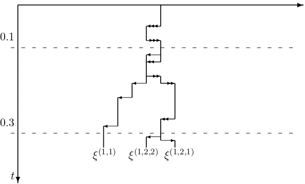
Figure 4 shows the trace of a possible realization of GI-RW, where the labeled grove coincides with the space of scaling exponents from Figure 1b.

✲

0.1

0.3

✛✛✛ ✲

✲✲

✛✛

✛

✲ ✲

✛ ✲✲

✛✛

✛ ✲ ✛

✛

Z

d

❄ t

ξ(1,1) _ξ(1,2,2) _ξ(1,2,1)

In section 2 we have stated our main result on the multiple scale analysis in terms of suitable rescaled finite dimensional marginals of a single BRW/SRW (recall Theorem 2). At this point we want to generalize this in an obvious way to the grove indexed systems of branching models: let (G, S) be a labeled grove, and consider the (G, S)-indexed system of SRW/BRW (recall the second example above). Following (2.37), we abbreviate

X(G,S)_:=_{Xe+

(29)

For a given space of scaling exponents, (T, A), recall from (2.33) the definition for a sequence of space-time points being on a (T, A)-scale.

(iv) Extended multiple scale analysis. Fix a labeled grove, (G, A), such that A_|_G− ≡0. Then a family of sequences of space-time pointsR_text∈(R

2 _×

R

+₎G+

∪(R

+₎G\G+ ,

Rext_t :=_{r_te+ := (y_te+, s_te+), e+_∈G+;se_t, e_∈G0_}, (3.18) is said to beon an extended (G,A)-scale iff the following three conditions hold: for alle+_{, f}+_∈

G+_,_e+_∧_f+_{6∈ {}_e+_{, f}+_}_,

log1_{∨ k}ye+ t −yf

+

t k2∨ |se + t ∨sf

+ t −se

+_∧_f+

t |

logt −→t→∞1−A(e

+_∧_f+_), _(3.19)

and in addition to (3.19), fore_∈G_\G−, lim t→∞

logse t

logt = 1, (3.20)

and for e, f _∈G,

se_t _≤sf_t, if e _≤ f. (3.21)

Remark. Given a grove, G,Rext_t equips Gwith the labeling function

St(e) :=set, e∈G\G+. (3.22)

(30)

Recall the definition ofα-block meansB(·,·),α_{from (2.13). We are now interested in the joint} dis-tribution of several of the objects indexed by a grove, i.e., we need to investigate the asymptotics of

L[BbRextt , α_{] :=}L

b

Bret+,α_; _e+∈_G+

. (3.23)

Based on that we state the following theorem. Below we define the suitable property of labeled trees one needs in order to conclude Theorem 2 as a particular case of Theorem 2(’).

Theorem 2 (’) (Multiple scaling extended on grove indexed SRW/BRW) Let Rext

t :={re + t := (ye

+ t , se

+

t ), e+∈G+;set, e∈G0} be on an extended (G, A)-scale. If Pθ :=_LΨ(θ)[_X(G,St)_], _(3.24)

then the following holds as t→ ∞: (Pθ)

(e+₀, ye + 0

t )

[_BbRextt , α∈·] =⇒ t→∞

P

0_[Y(e+₀),(G_,A∧(1−α)) _∈_·_]. _(3.25)

Notice that the concept of grove indexed branching processes includes the description of the finite-dimensional marginals of the single branching process. To see this, we define labeled trees with a special structure:

Definition 3 (Linearly ordered tree)

A labeled tree,(T, S), is refered to as linearly ordered iff for each subtree T′ ⊆T,

S(_∧e∈T′e) =∧_e_∈_T′S(e). (3.26)

Remark. Consider a sequence of linearly ordered trees, (T, St). Since its labels are such that St(e)∧St(f) =St(e∧f), (3.27) we obtain immediately that _|St(e)∨St(f)−St(e∧f)|=|St(f)−St(e)|.

Furthermore, if a family of space-time points Rt is on a (T, A)-scale, it is always possible to extend toRext_t by unitingRtwith a family of time points{set, e∈T0}such thatTequipped with Stgiven by (3.22) is linearly ordered. Thus, Theorem 2 follows immediately from Theorem 2(’).

✷

3.2 Moment formula for the tree indexed SRW

Fix a labeled binary tree, (T, S), a starting time, s∅, and letX be a version of a (T, S)-indexed SRW. Then the main aim is to obtain a graphical representation of an explicit formula for the space-time mixed moments of X(T_,S₎

(recall (3.17)).

(31)

all possible genealogical records, i.e., in particularG∈ GT+ (recall (3.3)), and is equipped with monotone labels, _{U(e); e _∈ G_}, such that the splitting time, U(e), from a possible common ancestor,e=e+_∧

Tf+, of the two individualse+, f+∈T+occurred latest before the branches

Xe+ and Xf+ started to follow an independent dynamic. To describe this formally, we need more notation.

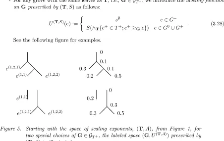
- For any grove with the same leaves as T, i.e.,G_{∈ G}_T+, we introduce the labeling function on G prescribed by (T, S) as follows:

U(T,S)(e) :=

(

s∅ e_∈G−

S(_∧T{e+∈T+;e+ ≥Ge}) e∈G0∪G+

. (3.28)

See the following figure for examples.

e(1,1)

❅❅ e(1,2,1)

❅❅

e(1,1) _e(1,2,2)

Figure 5. Starting with the space of scaling exponents, (T, A), from Figure 1, for two special choices of G∈ GT+, the labeled space (G, U(T,A)) prescribed by (T, A) is illustrated.

0 0.1 ❅❅

0.3 0.1

❅❅

0.2 0.5

❅❅

e(1,2,1) _e(1,2,2)

0.2

0 0.3 ❅❅

0.3 0.5

Furthermore

- For a given labeled grove, (G, U), withG_{∈ G}_T+, letξbe a version of a (G, U)-indexed RW. For s∅ _≥0,x∅ _∈Z

d_, _F_(T+_{) := (F}e+

;e+ _∈_T+_), _Fe+

∈M₀+(Z

d_), _S(T+_{) := (S(e}+_); _e+ _∈

T+), we set

S_s(G∅_,S,U₍_T)+₎[F(T

+_)](x∅_{) :=}_Eδ_x∅, s∅_[ Y e+_∈_T+

Fe+(ξ_Se+₍_e+₎)]. (3.29)

In particular, in the simplest case whereT:=_{∅,(1)_}has one leaf only,_S_s(∅G_,S,U₍_T)+₎ coincides with the semigroup Ss∅_,S₍₍₁₎₎ defined in (1.9).

- As motivated above, since (G, U) should represent the genealogy, later we want to integrate expressions of the form (3.29) about all possible labelingsU ofG_{∈ G}_T+ such thatU|_G−≡ s∅ and U_|_G+ =S|_T+. Fore∈G0∪G+, let

←

eG denotese’sdirected ’predecessor’, i.e., ←−

getdocf99b. 551KB Jun 04 2011 12:05:14 AM

Contents

1

Introduction

2

Cluster formation in two dimensions

3

Genealogical representation of SRW-functionals