MORPHISMS AND MODULES FOR POLY-BICATEGORIES
J.R.B. COCKETT, J. KOSLOWSKI, AND R.A.G. SEELY
ABSTRACT. Linear bicategories are a generalization of ordinary bicategories in which there are two horizontal (1-cell) compositions corresponding to the “tensor” and “par” of linear logic. Benabou’s notion of a morphism (lax 2-functor) of bicategories may be generalized to linear bicategories, where they are called linear functors. Unfortunately, as for the bicategorical case, it is not obvious how to organize linear functors smoothly into a higher dimensional structure. Not only do linear functors seem to lack the two compositions expected for a linear bicategory but, even worse, they inherit from the bicategorical level the failure to combine well with the obvious notion of transformation. As we shall see, there are also problems with lifting the notion of lax transformation to the linear setting.
One possible resolution is to step up one dimension, taking morphisms as the 0-cell level. In the linear setting, this suggests making linear functors 0-cells, but what struc-ture should sit above them? Lax transformations in a suitable sense just do not seem to work very well for this purpose (Section 5). Modules provide a more promising direction, but raise a number of technical issues concerning the composability of both the modules and their transformations. In general the required composites will not exist in either the linear bicategorical or ordinary bicategorical setting. However, when these compos-ites do exist modules between linear functors do combine to form a linear bicategory. In order to better understand the conditions for the existence of composites, we have found it convenient, particularly in the linear setting, to develop the theory of “poly-bicategories”. In this setting we can develop the theory so as to extract the answers to these problems not only for linear bicategories but also for ordinary bicategories. Poly-bicategories are 2-dimensional generalizations of Szabo’s poly-categories, consisting of objects, 1-cells, and poly-2-cells. The latter may have several 1-cells as input and as output and can be composed by means of cutting along a single 1-cell. While a poly-bicategory does not require that there be any compositions for the 1-cells, such composites are determined (up to 1-cell isomorphism) by their universal properties. We say a poly-bicategory is representable when there is a representing 1-cell for each of the two possible 1-cell compositions geared towards the domains and codomains of the poly 2-cells. In this case we recover the notion of a linear bicategory. The poly notions of functors, modules and their transformations are introduced as well. The poly-functors between two given poly-bicategoriesPandP′ together with poly-modules
between poly-functors and their transformations form a new poly-bicategory provided
P is representable and closed in the sense that every 1-cell has both a left and a right
The research of the first author is partially supported by NSERC, Canada, and of the third by NSERC as well as Le Fonds FCAR, Qu´ebec. Diagrams in this paper were produced with the help of the
XY-picmacros of K. Rose and R. Moore and thediagxymacros of M. Barr. Received by the editors 2002-03-20 and, in revised form, 2003-02-11. Transmitted by Ross Street. Published on 2003-02-14.
2000 Mathematics Subject Classification: 18D05, 03F52, 16D90.
Key words and phrases: Bicategories, polycategories, multicategories, modules, representation theo-rems.
c
J.R.B. Cockett, J. Koslowski, and R.A.G. Seely, 2003. Permission to copy for private use granted.
adjoint (in the appropriate linear sense). Finally we revisit the notion of linear (or lax) natural transformations, which can only be defined for representable poly-bicategories. These in fact correspond to modules having special properties.
Introduction
Linear bicategories [6] were introduced as a natural 2-dimensional extension of linearly distributive categories [7]. When compared to ordinary bicategories, the most striking feature is the presence of two “global” (as opposed to “local”, inside the hom-categories) compositions BA, B ×BB, C // BA, C or tensors (“tensor”) and (“par”, to remind us of the connection with Girard’s linear logic, even though we do not use his notation). These are subject to certain compatibility conditions. Together with their respective units⊤and⊥, they yield two bicategory structures on the same class of objects, 1-cells and 2-cells that display a high degree of symmetry.
There are many examples of linear bicategories (some of which are described in [6]). A motivating example for us was provided in [16]: the Chu construction applied to a closed bicategory with local pullbacks produces a linear bicategory. In this paper we provide a further generalization of the Chu construction (section 2) which shows how one may construct a (cyclic) poly-bicategory from an (arbitrary multi-)bicategory.
The appropriate morphisms between linearly distributive categories are the linear functors of Cockett and Seely [8, 3]; these can be generalized to linear bicategories in a straightforward manner [6]. A linear functor between linear bicategories actually consists of two coherently linked morphisms which agree on the 0-cells, one of which is lax with respect to tensor composition while the other is colax with respect to the par composition. An important concept in this context is the notion oflinear adjunction. 1-cells with a common left and right linear adjoint, or “cyclic linear adjoints”, lead to the consideration of “linear monads” that combine the one-sided concept of a monad with that of a comonad to form a self-dual notion. These may also be viewed as linear functors from the final linear bicategory 1 into the given linear bicategory in much the same way as a monad in an ordinary bicategory may be viewed as a lax functor with final domain. There are two possible choices for morphisms between linear monads: “linear natural transforma-tions”, generalizing lax natural transformations between morphisms (i.e. lax functors) of bicategories, or “linear modules”, generalizing the familiar notion of (bi-)module between monads.
avoided by dispensing with the global composition and considering “multi-2-cells” with a finite sequence of inputs, but just one output. This yields a 2-dimensional generalization of “multi-categories”, as introduced by Lambek [19], that (together with double cate-gories) is subsumed by Tom Leinster’s “fc-multi-categories” [20]. Parallel to Szabo’s [26] generalization of multi-categories to “poly-categories” (with finite strings of objects as inputs and outputs), it was natural to consider generalizing these “multi-bicategories” to “poly-bicategories”, and to use these to provide a smooth theory of modules in the linear setting. This had the additional appeal for us, in that tacitly we were already employing poly-bicategories in the circuit diagrams we used for reasoning about linear bicategories in [6].
Let us recall the “logical” origins of linearly distributive categories and linear bicate-gories. Initially Cockett and Seely had considered a sequent calculus (for the tensor–par fragment of linear logic) with an input–output symmetry: the desire to model Gentzen’s cut rule categorically then motivated the introduction of linearly distributive categories [7]. The definition proceeded via the poly-categories mentioned above. Although not ex-plicitly stressed in the definition [6], linear bicategories have a similar underlying (albeit 2-dimensional) structure. We introduce this in Section 1 under the name “poly-bicategory”. Gentzen’s cut then provides the “local” composition of “poly-2-cells”. In contrast to the situation for multi-bicategories, poly-bicategories provide a natural setting for a notion of adjunction. A corresponding calculus of Australian mates is available as well.
In Section 2, we adapt an insight of Claudio Hermida [13], who had, in particular, noticed that the coherence requirements for bicategories can usefully be expressed in terms of the universal multi-properties expected of composite 1-cells. In the same manner the coherence issues for linear bicategories can alternately be expressed in terms of the universal poly-properties expected of the global compositionsandand their respective units ⊤ and ⊥. We then recover linear bicategories as “representable poly-bicategories” with chosen representing poly-2-cells for all these universal properties.
Besides showing that linear monads in a linear bicategory B together with linear modules and their transformations form a poly-bicategory, we wanted to go further, not only by dropping representability requirements as far as possible, but also by generalizing from linear monads to arbitrary linear functors. In Section 3 we generalize the latter to “poly-functors” between poly-bicategories, which yield “poly-monads” when the do-main is restricted to 1. (An alternative description arising from cyclic adjoints requires representability.)
[1] under the name “polyad”. So the results in the present paper have implications which are not widely known even at the bicategorical level. We shall “track” the applications to the bicategorical level in a series of remarks.
We introduce poly-modules and their transformations in Section 4. The latter admit a cut operation, provided P is representable and every 1-cell has a left and a right ad-joint. In the representable case the last condition amounts to the closedness of P. In terms of circuit diagrams, the existence of all adjoints allows us to “bend wires out of the way”. In the multi-categorical setting, where fewer configurations for cuts are possi-ble, such “bending” is not necessary. Therefore here the representability of the domain multi-bicategory suffices to ensure that “multi-module transformations” may be cut. We then discuss general conditions under which this construction produces a representable poly-bicategory. In particular, we show how these conditions specialize for the case of linear monads to the representability of the codomain poly-bicategory and the existence of reflexive equalizers and coequalizers which are preserved, respectively, by the par and tensor.
Finally, in Section 5 we reconsider linear natural transformations, which we had aban-doned in favor of poly-modules. Their definition requires tensors and pars to be chosen in
P, so this is really only suitable for linear bicategories (rather than for poly-bicategories). IfPalso has all left and right adjoints, linear natural transformations give rise to certain cyclic adjoint poly-modules, thus placing them in a context which allows both composi-tions.
A fact [1, 12] that seems sometimes to be forgotten is that “whiskering” of lax natural transformations with a lax functor on the codomain side does not, in general, produce a lax natural transformation. We are grateful to an (anonymous) referee for pointing this out to us. The prospect of restricting attention to the linear counterparts of homo-morphisms (= pseudo functors) between bicategories and pseudo natural transformations (with isomorphisms as 2-cell components) in order to secure this composition of the trans-formations between linear morphisms, as in the tricategoryBicat[11], seemed like a very unattractive option. After all, the lax-ness of the components of a linear functor is an essential feature. This provided us with considerable motivation to develop the notion of a poly-module which could support two compositions in order to subsume linear natural transformations.
1. Poly-bicategories
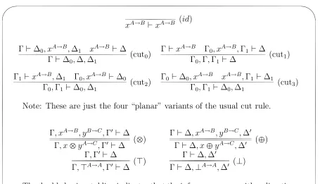
Let us recall the sequent rules for a logic of generalized relations between typed formulas A x // B that motivated the introduction of linear bicategories [6], cf. Table 1.
✬
✫
✩
✪ xA→B⊢ xA→B (id)
Γ⊢∆0, xA→B,∆1 xA→B ⊢∆
Γ⊢∆0,∆,∆1 (cut0)
Γ⊢xA→B Γ
0, xA→B,Γ1 ⊢∆
Γ0,Γ,Γ1 ⊢∆ (cut1) Γ1 ⊢xA→B,∆1 Γ0, xA→B ⊢∆0
Γ0,Γ1 ⊢∆0,∆1 (cut2)
Γ0 ⊢∆0, xA→B xA→B,Γ1 ⊢∆1
Γ0,Γ1 ⊢∆0,∆1 (cut3) Note: These are just the four “planar” variants of the usual cut rule.
Γ, xA→B, yB→C,Γ′ ⊢∆
Γ, xyA→C,Γ′ ⊢∆ ()
Γ⊢∆, xA→B, yB→C,∆′
Γ⊢∆, xyA→C,∆′ ()
Γ,Γ′ ⊢∆
Γ,⊤A→A,Γ′ ⊢∆ (⊤)
Γ⊢∆,∆′
Γ⊢∆,⊥A→A,∆′ (⊥)
The double horizontal line indicates that the inference may go either direction (top to bottom or bottom to top),i.e. these rules are “bijective”.
based just on the first five rules concerning the existence and local composition of poly-2-cells. The “bijective” rules may then be seen as additional representability requirements that imply the axioms for the two global compositions and the linear distributivities.
1.1. The definition of poly-bicategories. A poly-bicategory P consists of the data for a (2-)computad [23, 24], i.e.
1. a class P0 of 0-cells orobjects A, B . . .; 2. a directed graph over P0
P1
D0
/
/
D1
/
/ P0
with 1-cells f, g . . . x, y . . . as edges. As usual, their domains and codomains are indicated by single arrows, i.e. A x // B means D0x = A and D1x = B. This
graph freely generates a categoryF1 with typed paths Γ,∆, . . .as morphisms. The empty endo-path on an object A is denoted by ǫA. Given a path Γ of length |Γ|,
we write (Γ)i for its i-th component, (Γ)<i for its prefix of lengthi and (Γ)>i for its
postfix of length |Γ| −i−1, provided i <|Γ|; 3. a directed graph over F1
P2
∂0
/
/
∂1
/
/ F1
satisfying D0∂0 = D0∂1 and D1∂0 = D1∂1. We use double arrows to indicate
domains and codomains of the edges α, β . . ., called poly-2-cells, e.g., Γ α +3 ∆ means ∂0α = Γ and ∂1α = ∆. Among the edges we distinguish multi-2-cells with singleton paths as codomain and2-cells with singleton domain and codomain; together with
1. distinguished “identity 2-cells” x 1x +3
xfor each 1-cell x; 2. a partial operation (P2×)×(×P2)
; / P
2 calledcutthat mapsα, i,j, β to
(∂0β)<j, ∂0α,(∂0β)>j α,i;j,β +3 (∂1α)<i, ∂1β,(∂1α)>i, provided that
- i <|∂1α| and j <|∂0β|; - (∂1α)i = (∂0β)j;
- (∂1α)<i =ǫ implies (∂0β)<j =ǫ and (∂1α)>i=ǫ implies (∂0β)>j =ǫ.
To minimize the need for parentheses, we set αi: =α, iand jβ: =j, β.
These data are subject to three axioms:
(AS) cut is associative: if αi ; jβ and βk ; lγ are defined, then (αi ; jβ)i+k ; lγ = αi ;
l+j(βk ;lγ);
(IC) cut satisfies the interchange property (referred to as “commutativity” by Lambek [19]):
1. if αi ; jγ and βk ; lγ are defined and j < l, then αi ; j(βk ; lγ) = βk ;
|∂0α|+l(αi ;jγ);
2. if αi ; jβ and αk ; lγ are defined and i < k, then (αi ; jβ)k+|∂0β| ; lγ = (αk ;
lγ)i ;jβ.
The poly-bicategories Popand Pcoarise by reversing the 1-cells and the poly-2-cells of P, respectively.
1.2. Remark.
1. For any object A of P, the 1-cells from A to A with the appropriate poly-2-cells form a poly-category in the sense of Szabo [26].
2. Restricting any poly-bicategory to the 2-cells gives rise to an ordinary category. 3. A straightforward componentwise construction of the “product” of two structures
works for poly-bicategories: 0-cells and 1-cells are just pairs of 0- and 1- cells, and poly-2-cells in the product are pairs of poly-2-cells of the same “arity” m, n (i.e.
with m inputs and n outputs). There is a “singleton” poly-bicategory 1 consisting of one 0-cell, one 1-cell, and one poly-2-cell for every aritym, n. This “product” and “singleton” are in fact product and terminal object in the category pbcat defined in (3.3).
The need to keep track of the input and output positions makes the notation for multiple cuts rather unwieldy. Fortunately, as indicated in the introduction, planar circuit diagrams can be used to represent the constituents of poly-bicategories more efficiently. Objects correspond to areas in the plane. They are separated by non-intersecting labeled curve segments without horizontal tangents, called “wires”, corresponding to 1-cells from the domain on the left to the codomain on the right. Poly-2-cells are nodes with a certain number of input wires on top and output wires at the bottom. For notational convenience we enlarge these nodes to rectangular boxes carrying their labels inside. The 0-cell labels are usually left off to avoid cluttering the diagrams. Double wires indicate potentially non-empty typed paths inP1.
Γ0 Γ1 Γ2
Note that there is no provision for horizontally juxtaposing such diagrams.
The geometric content of associativity and interchange can likewise be clearly seen from the circuits; for example, associativity deals with circuit shapes like the following.
Γ0 Γ1 Γ2
Similarly, the interchange property refers to the parallel composition of two poly-2-cells with a third one, as illustrated by the following circuits.
Γ0 Γ1 Γ2 Γ3 Γ4
1.3. Examples.
1. If X is a category, the 0-cells and 1-cells of PX are the objects and morphisms, respectively, ofX. There exists a poly-2-cell between strings Γ and ∆ of composable 1-cells if and only if they have the same composite.
2. If X is a category, then its “suspension” ΣX has a single (unnamed) 0-cell, its 1-and 2-cells are the objects 1-and morphisms, respectively, of X.
3. Every bicategory and every linear bicategory is a poly-bicategory where all poly-2-cells happen to be 2-poly-2-cells. Recall that an example of a one object linear bicategory is a linearly distributive category, an example of which is any (not necessarily sym-metric) ∗-autonomous category.
Furthermore to any linear bicategoryBthere is a poly-bicategory whose poly-2-cells x:α1, α2, . . . , αn +3 β1, β1, . . . , βm
are 2-cells
α1α2· · ·αn 3+ β1 β2· · ·βm
inB. This poly-bicategory is essentially equivalent to B, which will be made more precise with the notion of “representability” in the next section.
4. Any setCof formal poly-2-cells (i.e.a computad) gives rise to a free poly-bicategory FpolyC by considering all formal composites. In fact, this is the category of circuits satisfying the non-commutative net condition (cf.below).
1.4. Multi-bicategories. Throughout this paper the reader should keep a parallel development in mind, viz. the notion of a multi-bicategory. The definition of a multi-bicategory is similar to that for poly-bicategories: the 2-dimensional structure has to be given by multi-2-cells only, and so the second interchange property must be dropped. Any poly-bicategoryP induces a multi-bicategory mP by forgetting all poly-2-cells which are not multi-2-cells or 2-cells. However, we do not wish to regard multi-bicategories just as specializations of poly-bicategories, since as far as morphisms are concerned, we will be interested in different ones in the two cases, cf. Section 3. The techniques and concepts are similar for the multi and poly cases, but generally one cannot derive results for one by a naive specialization, but ought to examine the full development more carefully. We have found the study of the poly case (which was necessary for a proper understanding of the “linear” case begun in [6]) to be helpful in understanding how the multi case ought to go, but we expect readers more familiar with ordinary bicategories will find the results on multi-bicategories of more immediate interest. Each section of the paper will include remarks pointing out the multi-bicategory development so that theme will be simple to follow.
1.5. Examples. Multi-bicategories
1. First, we note that to any bicategory B there is a multi-bicategory whose multi-2-cellsx:α1, α2, . . . , αn +3 β are 2-cellsα1α2· · ·αn +3 β inB. This
multi-bicategory is representable, and is equivalent toB. In this sense, multi-bicategories are the “right” (conservative) generalization of bicategories, poly-bicategories being the right generalization of linear bicategories.
2. Of course, “modules” and “multilinear functions” provide one of the prime examples for multi-bicategories. The roots of such examples go back at least to Bourbaki [4]. More specifically: rings with unit may be viewed as the objects of a multi-bicategory with left-R-right-S-bi-modules (ormodulesfor short) as 1-cells fromRtoS. Such a module M comes equipped with a left-actionRM µ∗ +3 M and a right-action MS µ∗ +3 M, subject to the familiar axioms. Heredenotes the tensor product of the underlying Abelian groups. Multi-2-cells from Mi:i < m to N are given
by multi-linear functionsfromM0,M1,· · ·,Mm−1 toN. This is a well-known and simple notion, which only becomes complicated when one tries to represent such functions by the tensor: then one characterizes them as homomorphisms of Abelian groups equalizing the m homomorphisms from M0 R0 M1 · · · Rm−2 Mm−1 to M0M1· · ·Mm−1 induced by the left and right actions, as well as module homomorphisms with respect to the left action of M0 and the right action of Mm−1, cf. [13]. Note then that the multi-bicategory structure is more natural than the bicategory structure with the tensor; in the present context, the latter amounts to the representability of the multi-bicategory (Section 2). Separating these notions (multi-linear functions and tensors, or more generally, multi-2-cells and representability) allows one to consider contexts where multi-linear functions occur, but (e.g.because of insufficient cocompleteness) cannot be represented by a tensor.
Since rings with unit are just monads inab, the monoidal category of abelian groups, and since monoidal categories are just one-object bicategories, this example admits a generalization to monads in any bicategoryBand modules between such. In fact, this can be generalized still further by replacing monads by unstructured endo-1-cells of B. The notion of module still makes sense in this context. The lack of identity modules in this construction motivated the introduction of interpolads in [15].
Another direction of generalization opens up when monads are replaced by arbitrary lax functors A // B (Section 4).
A 1-cell B x // C together with a poly-2-cell Γ, x α +3
∆ is called a right extension
orright hom of ∆ along Γ, if cuttingα with multi-2-cells at x induces bijections Γ,Θ +3 ∆
Θ +3 x
A right extension x, α is called absolute, if cutting α with poly-2-cells at x induces bijections
Γ,Θ +3 ∆,Ω Θ +3 x,Ω
Right extensions inPop,Pco andPcoop are calledright lifting, left extensionandleft lifting
in P, respectively, or left hom, right cohom and left cohom. We call P closed, if absolute right extensions and absolute right liftings exist for all typed paths with common domain, or codomain, respectively. If confusion with the notion of “closed” for bicategories is likely (see Remark 1.9), we shall say “poly closed” to emphasize the poly notion.
Since right extensions are unique up to isomorphic 2-cells, we usually denote them by Γ−◦∆,ev.
A f // B is left linear adjoint to B g // A, f ⊣ g, if poly-2-cells ǫ
A τ +3 f, g, the
unit, and g, f γ +3 ǫB, the counit, exist such that
f
f
g : =
f
f τ
γ
g ≫
f
f
1f and
g
g
f : =
g
g τ
γ
f ≫
g
g
1g (4)
To avoid excessive cluttering, we have left off the unit and counit boxes. We write f ⊢⊣g to indicate that f and g are mutually, or cyclic, linear adjoint, i.e. f ⊣g and g ⊣ f.
Since linear adjoints are determined up to isomorphic 2-cell, specific calculations re-quire a choice. Usually we denote a chosen left (right) linear adjoint of f by ∗f (f∗). If
every 1-cell in P has both a left and a right linear adjoint, we say that P has all linear adjoints.
The characterization by Street and Walters [25] of adjunctions by means of absolute right extensions or absolute right liftings carries over to the poly-setting for linear adjoints as well.
1.7. Proposition. A poly-2-cell g, f γ // ǫ
B is the unit of a adjunction f ⊣ g if and
only if f, γ is an absolute right extension of ǫB along g. So P has all linear adjoints if
A calculus of “Australian mates” [14] is available as well. If Γ1 and ∆0 consist of left adjoint 1-cells, then by a right mate for a poly-2-cell Γ0,Γ1 α +3 ∆0,∆1 we mean a poly-2-cell ∆∗
0,Γ0 β +3 ∆1,Γ∗1 such that the sequential composition with the units of ∆0 ⊣∆∗0 and the counits of Γ0 ⊣ Γ∗0 yields α, i.e.
Γ0 Γ1
∆0 ∆1
α =
Γ0 Γ1
∆0 ∆1
β (5)
Here (ǫA)∗: =ǫA and (x,Γ)∗: = Γ∗, x∗ for some choice of right adjoints.
If Γ and ∆ consist of cyclic adjoint 1-cells, a poly-2-cell Γ α +3 ∆ is called cyclic, if its left mate and its right mate from ∗∆ = ∆∗ to ∗Γ = Γ∗ agree. We call P cyclic, if all
1-cells are cyclic adjoints and all poly-2-cells are cyclic.
Clearly, the right mate β above is obtained by sequentially composing α with the counits of ∆0 ⊣ ∆∗0 and with the units of Γ0 ⊣ Γ∗0.
1.8. Examples.
1. If X is a groupoid, then PX has all linear adjoints. However, FpolyCdoes not have all linear adjoints, nor does the following example Hn.
For each n ≥ 0, the poly-bicategory Hn has one 0-cell ∗. Its 1-cells are given by
the oriented hyperplanes of Ê
n. These can be parametrized by elements (n, d) of Sn−1×
Ê, where S
n−1 ⊆
Ê
n
is the unit sphere. The hyperplane then consists of the vectorsx satisfyingx·n=d, the origin’s distance from the hyperplane being−|d|. There is a poly-2-cell from a sequence (ni, di):i > p to a sequence(n′j, d′j):j < q
if and only if the set of all vectors x∈Ê
n
satisfying
x·ni < di for i < p and x·n′j ≥d
′
j for j < q
is empty. Geometrically this means that the intersection of the regions “below” the input hyper-planes does not meet the intersection of the regions “above” the output hyper-planes. The cut operation works, since the regions in question (intersections and unions of half spaces of the form x·n < d) form a distributive lattice.
Given a multi-bicategory M, the objects of Chu(M) are endo-1-cells of M. The new 1-cells fromA a // AtoB b // B are so-called “Chu-cells”F=f0, ϕ0, f1, ϕ1
given by two independent multi-2-cells
f0 f1
It might be simpler to view F as the following diagram, which makes sense if M is
a bicategory.
There is a “negation” operator which interchanges the roles off0andf1: for example
F⊥ =
(technically, this is the requirement that it be representable for tensor units, in the sense of Section 2; certainly this is the case if M is a bicategory), then there are “unit” Chu-cells (which in fact represent the tensor and par units in Chu(M))
(for i < n), to the empty sequence, given byn multi-2-cells ρi inM
Note that An=A0 andan =a0 is forced by the typing. These multi-2-cells have to
satisfy these n equations:
It is now a straightforward exercise to show thatChu(M) is a cyclic poly-bicategory. (The cyclicity is “built-in” by having the cyclic set of multi-2-cellsρin the definition of a Chu-band.)
Remark: What if we use all 1-cells of M, and not just the endo-1-cells? The construction above can be carried through, but loses its essential character, since the result is only a multi-bicategory, and is no longer cyclic. The new 1-cells from A a // A′ to B b // B′ are F = f0, ϕ0, f1, ϕ1, f2 where f2 replaces the second
occurrence of f0 in the poly version; if M is a bicategory, this could be given dia-grammatically as follows.
of n+ 2 multi-2-cellsρj in M with domains the connected n-element substrings Γi
of the (2n+ 1)-element string
counted from the left. The 1-cellsk0,f1(0), . . . , f1(n−1),k2 serve as codomains. These multi-2-cells have to satisfyn+ 1 equations of the same “shape” as for the poly case. A new multi-2-cell into Kwith empty domain only makes sense ifK is an
endo-Chu-cell onA a // A. Then such a multi-2-cell consists of multi-2-cellsǫ
A ρ0 +3 k0 and
ǫA ρ2 +3 k2 together with a 2-cellk1 ρ1 +3 a subject to the evident equation.
1.9. Remark. Linear adjoints are not the same as ordinary adjoints. For example, linear adjoints can be defined in a poly-bicategory, but ordinary adjoints require representability (Section 2): they can only be defined in a representable multi-bicategory. There are other significant differences as well. Consider for example that sets, relations and inclusions may be viewed as a bicategory in two ways, differing in the global composition: forR⊆A×B and S ⊆B×C we can define
RS ={ x, z | ∃y.x, y ∈R∧ y, z ∈S} RS ={ x, z | ∀y.x, y ∈R∨ y, z ∈S}
This means that we can consider this either as a linear bicategory [6] by combining both bicategory-structures into a whole, or as a “degenerate” linear bicategory in one of two ways, where both global compositions are given by , or by . As a bicategory with global composition , rel is closed in the sense that right liftings and right extensions exist in the sense of Street and Walters [25] (these were called left and right homs in [6]), but it is not poly closed. Only functions have right adjoints (are “maps”). As a bicategory with global composition, relis coclosed, but not poly coclosed. Finally, as a linear bicategory with the global compositionsand ,rel has all linear adjoints: every relation R is a cyclic linear adjoint with ¬R◦ as two sided linear adjoint. In particular,
now rel is poly closed and cyclic.
1.10. Poly-monads. The concept of amonadT=x, µ, ηon an object can be
formu-lated in a multi-bicategory: T consists of an endo-1-cell A x // A, the carrier, together
with multi-2-cells x, x µ +3 x, the multiplication, andǫA η +3 x, the unit, subject to the obvious axioms. In the poly-setting however, we need a more symmetric “linear” notion that combines a monad and a comonad on the same object. As was shown in [6], we can think of a poly-monad (a “linear monad” in the representable setting of Section 2) in at least two ways. Concretely, a poly-monad consists of endo-1-cells f⊗, f⊕, on some objectA which have the structure of a monad and a comonad, respectively, together with actions and coactions
f⊕
, f⊗ ν ⊕
L
+
3 f⊕ ks ν ⊕
R f⊗
, f⊕
f⊗
, f⊕ ks ν ⊗
L
f⊗ ν ⊗
R
+
3 f⊕ , f⊗
A simple example of a poly-bicategory with a poly-monad is given by S1 (cf. sub-section 3.3): there is one 0-cell ∗, two 1-cells ⊤,⊥, and infinitely many poly-2-cells con-sisting of all strings x1, . . . , xn +3 y1, . . . , ym where either all x’s and at most one y
are ⊤, or all y’s and at most one x are ⊥. The monad is given by ⊤,⊤ +3 ⊤ ks ǫ, the comonad by ⊥,⊥ ks ⊥ +3 ǫ. The actions are given by ⊥,⊤ +3 ⊤ ks ⊤,⊥ and by ⊤,⊥ ks ⊥ +3 ⊥,⊤. This poly-monad is “generic”; i.e. S1 is initial among all nullary representable (cf. Section 2) poly-bicategories with respect to morphisms (cf.
3.3).
In the presence of de Morgan duality (e.g.if P is a ∗-linear bicategory), the comonad structure on f⊕=f⊗∗ is determined as the mate of the structure on the monad f⊗, and
vice versa, and the actions and coactions are derivable. So the notion of a poly-monad incorporates the duality in the poly setting that is inherent in the de Morgan setting.
For example, a monad in rel is a preorder relation on the set. Its de Morgan dual is an anti-reflexive, anti-transitive relation: i.e. x, x is never in ¬R◦ and x, y in ¬R◦
only if for all z either x, z or z, y is in ¬R◦. Such a relation under the par provides
a comonad (the par unit is the largest anti-reflexive relation). Notice there is an action (¬R◦)R ≤ (¬R◦) as x, y ∈ ¬R◦ and y, z ∈ R cannot have z, x ∈ R otherwise
(using the transitivity of R)y, xwould be in R which by assumption it is not.
2. Representability
We now turn to the question to what extent the 2-cells of a poly-bicategory already determine the whole structure. The idea is to bundle all inputs and all outputs of a poly-2-cell α into single 1-cells, respectively, arriving at a 2-cell that “represents” α. Abstracting away from individual poly-2-cells, there should be two bundling operations for typed paths, one for inputs and one for outputs. These may then be viewed as two global compositions of 1-cells and 2-cells.
The idea of clarifying coherence requirements by employing universal properties to define global compositions has been proposed by Hermida,cf.Section 8 of [13]. Although intended as a tool for attacking the problem of defining weak n-categories, where even the formulation of the correct coherence requirements had stalled progress beyond n= 3, its benefits are already available in the 2-dimensional setting.
2.1. Representability in poly-bicategories. A multi-2-cell Γ π +3 x is said to
represent the typed path Γ as input, if cutting with π atx induces bijections as follows. Γ0,Γ,Γ1 +3 ∆
Γ0, x,Γ1 +3 ∆
(9)
Dually, a comulti-2-cell y σ +3 Γ represents Γ as output, if cutting with σ at y induces an analogous bijection.
A poly-bicategory is called representable, if each typed path is representable as input and as output. It is calledbinary representable, if this holds for all paths of length 2, and
nullary representable if it holds for all empty paths.
Clearly, representing (co-)multi-2-cells are unique only up to composition with an isomorphism. But singleton paths admit a canonical representation by means of their identity 2-cells. Due to the naturality requirement, it is clear that representability for typed paths of lengths 0 and 2 implies representability of all paths.
The relationship between representable poly-bicategories and linear bicategories re-sembles that between fibrations and pseudo-functors into Cat. The first notion together with a choice of “structural data” induces the second notion. However, as soon as we make such a choice, there will be implied coherence conditions.
A chosen representing multi-2-cell for a typed pathx, ywill be denoted byx, y
+
3 x y and its codomain will be called “the tensor” of x and y. For an object B, a chosen representing multi-2-cell for ǫB will be written as ǫB ⊤ +3 ⊤B and its codomain will be
called “the tensor unit” of B. The dual notions are xy
+
3 x, y and ⊥B ⊥ +3 ǫB
with “the par” of x and y, respectively “the par unit” of B, as domain.
By abuse of terminology, we say that P has tensors or has tensor units, respectively,
has pars or has par units, if the corresponding representing (co-)multi-2-cells exist and some choice has been made. The ability to make such a choice of course presupposes a sufficiently strong choice principle.
The corresponding nodes in a circuit diagram will be calledtensor (par) links andunit links. In logical terminology, these correspond to introduction rules for and ⊤, and to elimination rules for and ⊥:
x y
xy
(I) and
⊤B
⊤ (⊤I) respectively
xy
x y
(E) and
⊥B
⊥ (⊥E) (10)
2.2. Theorem. If P is a poly-bicategory that has tensors, pars and their units, then its objects, 1-cells and 2-cells together with the chosen data form a linear bicategory B in the sense of [6].
Proof. In the one-object case, this is in the original paper on linearly distribu-tive categories [7], and the general proof is essentially the same. We just mention that cutting appropriate tensor and par links induces poly-2-cells f, gh +3 f g, h and f g, h +3 f, ghwhenever D1f =D0g and D1g =D0h. Under the inverse bijections of (9) and its dual, these yield the “linear distributivities”
characteristic of linear bicategories.
2.3. Proposition. For an object B, any representing multi-2-cell ǫB ⊤ +3 ⊤B for ǫB as input and any representing comulti-2-cell ⊥B ⊥ +3 ǫB for ǫB as output are cyclic
mates.
Proof. There exist uniquely determined 2-cells ⊤B,⊥B γ +3 ǫB ks γ
This immediately establishesτandγas the unit and counit of an adjunction⊤B ⊣ ⊥B,
and similarly τ′ and γ′ as unit and counit of an adjunction ⊥
B ⊣ ⊤B.
Conversely, if a representing multi-2-cellǫB ⊤ +3 ⊤B forǫB as input is cyclic, i.e. ⊤B
is a cyclic adjoint and both mates of the multi-2-cell agree, then the mate is a representing comulti-2-cell for ǫB as output.
Note this makes ⊤B,⊥B a linear monad.
The “negation links” introduced by Schneck [22] in order to adapt the Rewiring Theo-rem [2] to the non-commutative setting, represent the units and counits of the adjunctions (11).
Linear adjoints for representable poly-bicategories correspond to linear adjoints for linear bicategories [6]. In that paper we gave an analysis of linear and cyclic adjoints, of various notions of closed structure, including the “right” generalization of ∗-autonomous categories to this setting. For all this, and (anticipating the next section) for a discussion of (linear) monads, we refer the reader to that paper.
In a closed poly-bicategory, representability for tensor is equivalent to representability for par, and each may be given in terms of a simple universal property. To see this we need to construct certain slice categories of a bicategory.
LetPbe a poly-bicategory: then byP/Γ we mean the slice category whose objects are comulti-2-cellsZ v +3 Γ and whose maps v f // v′ are 2-cellsZ f +3
Z′ withf ;v′ =v.
Dually, by Γ/P we mean the coslice category whose objects are multi-2-cells Γ v +3 Z and whose maps v f // v′ are 2-cells Z f +3
Z′ with v ;f =v′.
2.4. Lemma. For a closed poly-bicategory P, the following are equivalent.
1. P is tensor and tensor unit representable.
3. the coslice category [A, B]/P has an initial object for all composable 1-cells A and
B, and the coslice category ǫX/P has an initial object for each 0-cell X.
4. the slice categoryP/[A, B]has a final object for all composable 1-cellsAandB, and the slice category P/ǫX has a final object for each 0-cell X.
Proof. The equivalence (1) ⇔ (2) is an easy consequence of de Morgan duality; the equivalence (2) ⇔ (4) is dual to the equivalence (1) ⇔ (3). So we shall sketch that last equivalence only.
Clearly the representing objects for the empty and binary sequents must satisfy these conditions. For the converse of the binary case we have the following equivalences:
C1, .., Cn, A, B, C1′, .., Cm′ +3 Z C2, .., Cn, A, B, C1′, ..., Cm′ +3 C1−◦Z
.. . A, B, C′
1, . . . , Cm′ +3 (Cn−◦ · · · −◦Z)
.. .
A, B +3 ((Cn−◦ · · · −◦Z)◦− · · · ◦−Cm′ ) AB +3 ((Cn−◦ · · · −◦Z)◦− · · · ◦−C′
m)
showing that an initial object in the coslice category does give a representing object. The nullary case may be left to the reader.
Often poly-bicategories are naturally closed while their representability is a somewhat more artificial property. The well-known example of the tensor for Abelian groups (or any commutative theory) bears witness to this.
2.5. Examples.
1. 1 is representable (since all the poly-2-cell hom sets are singletons). As a linear bicategory, 1 has just one 0-cell, one 1-cell, and one 2-cell.
2. The (componentwise) “product” of two representable poly-bicategories is repre-sentable.
3. S1 (subsection 1.10) is nullary representable, but not binary representable. For example, there is no object ⊤⊤ representing ⊤,⊤ as output. Some strings are always representable, however: for example, ⊤,⊥ is representable as output (i.e.
4. In the poly-bicategory Chu(M) of Example 1.8(2), representing multi-2-cells exist for empty typed paths (as input), provided this is the case inM, as we pointed out. To guarantee the existence of representing multi-2-cells for typed paths of length 2, the existence of these in M does not suffice. One also needs to require the 2-cells of M to admit right extensions (or right homs) −◦ and right liftings (or left homs) ◦− (i.e. to be closed in the sense of Street and Walters [25]) as well as local pullbacks. Then for Chu-cellsF=f0, ϕ0, f1, ϕ1 fromA a // Ato B b // B
and G = g0, γ0, g1, γ1 from b to C c // C the central 1-cell of their tensor f0 g0, η0, e1, η1 is the pullback of the cospan
g0−◦f1 g0−◦ϕ◦−1 +3 g0−◦b◦−f0 ks γ0−◦◦−f0 g1◦−f0
cf. [17] and [16]. (The superscripts indicate exponential transposes.)
2.6. Remark. Representability is a significant property which may well require non-trivial conditions on the structures concerned. In Section 4 we shall study module poly-bicategories, and for them to be representable will require strong hypotheses on the un-derlying poly-bicategories, even if they are representable themselves. For now, we can present a simpler illustration of a construction which may destroy representability. Fur-thermore, this construction attempts to capture the essence of dinaturality, but to explore that further would take us beyond the scope of this paper.
For a poly-bicategory P we construct a new poly-bicategorytwist(P) with the same objects asP. Each 2-cellx α +3 yofPinduces two 1-cells +αand −αintwist(P), with domainD0x=D0y and codomain D1x=D1y.
Now a poly-2-cell ωL, ωR in twist(P) between two strings of signed 2-cells consists
of two poly-2-cells inPsubject to the requirement that the parallel composite of ωLwith
all positive inputs and all negative outputs agrees with the parallel composite ofωR with
all negative inputs and all positive outputs.
The following example of a poly-2-cell from +α,−β,+γ to +δ,+η,−ϕ illustrates the typing of ωL and ωR.
a b c
d′ e′ f′
α γ
ω+
ϕ
a′ c′
f
=
a b c
d′ e′ f′
β
ω−
δ η
b′
d e
(12)
A cut ofωL, ωRand another pairψL, ψRwith−ϕas the first component in its domain
2.7. Circuits for representable poly-bicategories. We wish to display the inverse bijections of (9) (from top to bottom) in our circuit diagrams. The elimination rules for and ⊤ and the introduction rules for and ⊥ require new devices, called
switching links and thinning links, respectively. These are not poly-2-cells, hence we distinguish them by their round shape:
xy
These links must not occur freely in a well-formed circuit diagram but have to be “attached” somewhere. In the binary case, the wires enclosing the dot have to be inputs of some (composite) poly-2-cell such that the resulting region is closed. Conversely, every closed region has to contain precisely one dot. This is theregion criterion of Schneck [22]. Moreover, a diagram corresponding to a poly-2-cell has to satisfy the net condition [2]: for each switching link opening one of the non-tensored wires has to yield a connected acyclic graph.
For the tensor unit ⊤B, we need to require that both ways of defining the bijections ⊤B,⊤B +3 ⊤B
⊤B +3 ⊤B
and x,⊤B, y +3 xy x, y +3 xy
agree, and dually for⊥B. To indicate, which of the two variants is intended, we connect
the loop of the dotted “lasso” in a thinning link with the appropriate neighboring 1-cell wire, resulting in nodes that correspond to elimination rules for ⊤ and to introduction rules for ⊥.
Diagrams with lassos have to remain planar. If there are several possible targets for a lasso, any one of them may be used. This is the essence of the “Rewiring Theorem” of [2] that concerns the possible “moves” of the lasso loop. Even vertical moves across switching links are allowed, but moves between non-tensored wires of a switching link are ruled out.
system:
Similarly, there are local “reductions” of the form
x y
together with their duals. Notice that the left diagram only makes sense as part of a larger diagram, since the region criterion is not satisfied.
2.8. Representability in multi-bicategories. What does “representability” mean in the context of multi-bicategories? Of course we need only half the representability: in a multi-bicategory only the inputs of the multi-1-cells need to be bundled, resulting in just one global composition. So, a multi-bicategory is calledrepresentable, if each typed path is representable as input. The development in the multi setting is essentially the same as it was above for the poly setting, so we shall only make a few comments here where there are distinctions the reader ought to be aware of, and end with a few examples.
Although every multi-bicategory is also a poly-bicategory, here the notion of repre-senting non-singleton paths as outputs is not interesting. Hence our slightly overloaded terminology should not lead to misunderstandings. But note that there is a subtlety in our definition, because of the “contextual” presentation. Multi-2-cells representing a path as input correspond to Hermida’s [13] “strongly universal” multi-2-cells, rather than to his “universal” multi-2-cells which satisfy a non-contextual version of the requirement above,
i.e. without parameters Γ0 and Γ1.
Theorem 2.2 has an analogue for representable multi-bicategories that have tensors and tensor units: for such a multi-bicategory, its objects, 1-cells and 2-cells together with the chosen representability data form a bicategory B. Likewise Lemma 2.4 has an analogue, which essentially amounts to dropping those clauses which refer to the comulti (par) structure.
2.9. Examples. Representability in multi-bicategories.
1. The multi-bicategory of endo-1-cells and modules over a bicategory B (Example 1.5(2)) usually fails to have representing multi-2-cells for empty paths (as inputs). The minimal amount of structure on an endo-1-cell that would rectify this shortcom-ing is a “multiplication”bb β +3 b that is a coequalizer of 1bβ and β1b (and
hence in particular associative). This leads to the notion of “interpolad” introduced in [15]. Of course, the relevant modules now have to be compatible with this multi-plication. Monads happen to be interpolads with additional structure (units), hence in this case representing multi-2-cells for empty paths also exist. This specializes to the case of (bi-)modules between rings.
To have representing multi-2-cells for paths of lengths 2 between endo-1-cells, or interpolads, or monads in a bicategoryB, we need the existence of local coequalizers and their preservation by the horizontal compositionofB. The latter is certainly guaranteed ifBis closed. In all three cases, the preservation of local coequalizers by
then allows us to build representing multi-2-cells for longer paths by composition,
i.e. cut.
2. In analogy to the situation for modules over a fixed ring, for so-called “concrete categories” of structured sets, tensor products have been defined by a non-contextual version of the universal property (9), i.e. without the parameters Γ0 and Γ1, cf. [10]. While such tensor products exist, e.g., in any variety, the associativity of the corresponding binary operation is not automatic. Davey and Davis [10] show that associativity holds in so-called “entropic” varieties (where every operation is a homomorphism), but claimed not to know any non-entropic variety where this is the case. However Whitney knew that this tensor product was associative in groups (manifestly non-entropic) [oral communication by Fred Linton]. In other cases this tensor may be non-associative.
3. If X is a category, Span(X) is a comulti-bicategory; the usual requirement that X needs pullbacks is only necessary for representability. Of course, Span(X) is representable if X has pullbacks, via the usual construction.
3. Poly-functors and morphisms between poly-bicategories
Recall that one motivation for linearly distributive categories was the desire to relate the tensor and par of linear logic in the absence of a negation and hence of de Morgan duality. The same kind of reasoning can lead to the notion of linear functor [8]: a lax functor F between ∗-autonomous categories by de Morgan duality has an oplax companion. In the linearly distributive case, this companion cannot be derived but has to be given explicitly. Similar considerations apply in the 2-dimensional setting. A linear bicategory B may be viewed as supporting two bicategory structures B⊗
and B⊕
are the linear bicategories induced by poly-bicategories P and P′ with tensors, pars and units, then linear functors consist of a lax functor B⊗ F⊗
/
/ B′⊗ and an oplax functor
B⊕ F⊕
/
/ B′⊕, required to be “mutually relatively strong”. This means there have to be natural transformations
The compatibility requirements turn out to be highly poly-bicategorical in spirit. From this point of view, it is clear that the notion of linear functor is well suited to the poly-bicategorical setting. The key is thatF⊗does not operate on plain poly-2-cells, but rather on poly-2-cells with a chosen output position (like the first factor of a cut). In particular, poly-2-cells with empty output cannot occur as arguments ofF⊗. Dually,F⊕ operates on poly-2-cells with chosen input position (like a second factor of a cut).
3.1. Poly-functors. A poly-functor P F //
P′ consists of 1. an object function P0 F // P′0;
2. directed graph morphisms P1 F ⊗
of P′. These are presented by so-called functor boxes
Γ
The image of the selected wire, called theprincipal wire, leaves or enters the functor box at the principal port, marked by a little half circle for easy reference. It can always be deduced from the typing information. (The wire labels inside the functor boxes, here left off for space reasons, are the same as in P.)
(IF) identity 2-cells are preserved, i.e. F⊗1
x0 = 1F⊗x and F⊕01x = 1F⊕x;
(CF) cut is “preserved” in the sense that a cut of two functor boxes can be rewritten as a functor box containing a corresponding cut. This subsumes the notion of F⊗ and F⊕ preserving certain cuts and of being mutually strong, i.e. F⊗ acts on F⊕, and F⊕ coacts onF⊗. In other words, functor boxes can be “absorbed” along their principal wires.
(plus other symmetric cousins of these rules [8, 6])
If both Pand P′ have tensors and their units, the graph-morphismF⊗ becomes a lax functor with respect to and ⊤. The structural 2-cells are given by
F⊗xF⊗y
Dually, F⊕ becomes a colax functor if both Pand P′ have pars and their units. If P and P′ are representable then F restricts to a linear functor. In particular, F⊗ and F⊕ are mutually strong.
We denote bypbCatthe large category whose objects are poly-bicategories and whose morphisms are poly-functors. (The latter sections of this paper shall consider what higher dimensional structure might be appropriate in this context.)
3.2. Examples.
1. A poly-functor 1 // P is a poly-monad [6].
functor. Furthermore, if the category has the ! modality, the ? modality may again derived via de Morgan duality. As ! is monoidal, =!, ? naturally forms a linear functor. Similarly, if V has binary products, the functor V×V × // V is monoidal and together with its de Morgan dual, the binary coproduct functor, constitutes a linear functor ×,+.
In [8] it was shown that these three linear functors may be defined in a symmetric linearly distributive category, where in general the two components will not be linked by de Morgan duality.
3. For a linear bicategoryB, itslocal powerB[2] has the same 0-cells but hom-categories
B[2]A, B = BA, B ×BA, B. The components of the obvious “diagonal” lin-ear functor B ∆ // B[2] agree on 0-, 1- and 2-cells. Binary local products and coproducts then are simultaneously provided by a linear functor (pseudo-)adjoint to ∆.
4. The functor parts of a linear functor may be trivial so that the structure is carried by the natural transformations alone. The following example is due to Retor´e [21]: Let Coh be the ∗-autonomous category of coherence spaces, with the usual ,. (So objects are pairs A = SA, RA consisting of a set SA and a symmetric,
anti-reflexive relation RA.) Define another “lexicographic” tensor structure on Coh as
follows:
AB =SA×SB,{ (a, b),(a′, b′):bRBb′ orb=b′∧aRAa′}
Then one may show that the identity functor is a linear functor from Coh with the (degenerate or compact) linear structure given by to Coh with the linear structure ,.
5. Given symmetric ∗-autonomous categories X, Y with coproducts (and therefore products), any lax functor X F // Y induces a linear functor F, F⊥ (where F⊥
is the de Morgan dual of F) [8, Proposition 5], and hence a linear functor between the linear bicategories of matrices of X and Y, respectively (cf.[6, section 1.2]).
3.3. Morphisms of poly-bicategories. Besides this comparatively elaborate notion, a simpler one is available:
A morphism P F
/
/ P′ between poly-bicategories assigns objects, 1-cells and poly-2-cells of P′ to those in P such that identity 2-cells and cuts are preserved. The resulting large category is denoted by pbcat.
Note that pbcat has componentwise products, equalizers, and a terminal object1, as we pointed out in Remark 1.2 (3); their construction is simple and standard.
The following construction provides a formal way of selecting one of the inputs or outputs of all poly-2-cells, as required by the notion of poly-functor. This enables us to reduce the notion of poly-functor to that of morphism of poly-bicategories.
For a given poly-bicategory P, a new poly-bicategory SPwith the same objects as P
is specified as follows:
1. each 1-cell f of Pinduces two 1-cells +f and −f inSPwith the same domains and codomains as f has in P;
2. each poly-2-cell Γ α +3 ∆ of P induces |Γ| poly-2-cells i, α, i < |Γ|, in SP that have the positive copies of α’s inputs as inputs, except in position i, where the negative copy ofα’s input occurs. All outputs are the negative copies ofα’s outputs. Similarly, there are |∆| poly-2-cells α, j, j < |∆|, with one exceptional positive output in position j.
Notice that a wire along which a cut is performed inSPis an exceptional input or output for precisely one of the involved poly-2-cells, hence the resulting poly-2-cell has again one exceptional input or output. We have already seen a special case of this construction as S1 (subsection 1.10).
3.4. Proposition.
1. There exists a morphismSP S0 //
P that preserves objects and forgets the signs of the 1-cells as well as the selected inputs or outputs of the poly-2-cells.
2. There exists a morphism SP S2 //
SSP that preserves objects, doubles the signs of the 1-cells and re-selects the exceptional inputs or outputs of the poly-2-cells.
3. S,S0,S2 constitutes a comonad on pbcat.
4. Poly-functors P // P′ between poly-bicategories are in bijective correspondence
with morphisms SP // P′, i.e. with arrows in the coKleisli-category pbcatS of
the comonad S. Hence pbcatS ≃pbCat.
Proof. (1), (2), (4): Immediately clear.
(3): The coassociativitiy follows, since the tripling of signs can be achieved by first doubling them and then doubling either the first of the second copy again. Similarly, first doubling the signs and then forgetting either the first or the second copy results in the identity.
We can also characterize morphisms in terms of poly-functors: morphisms P G // P′
are in bijective correspondence with poly-functors P G⊗,G⊕
/
/ P′ for which the graph morphisms G⊗ and G⊕ agree also on edges and the assignments of poly-2-cells are inde-pendent of the selected input or output position.
3.5. Multi-functors and multi-bicategories. There is a notion of “multi-functor” which plays the same role for multi-bicategories as poly-functors play for poly-bicategories, but it is in fact a familiar notion, viz. the multi version of the ordinary notion of lax functors (or simply “morphisms”) of bicategories. The circuit boxes for such lax functors are described in [8], where they are called “monoidal functor boxes”. These have only the principal output port through which the sole output wire of a multi-2-cell leaves the box. We have already seen (Lemma 2.4) that the existence of adjoints introduces a con-nection between the “tensor” (input) and “par” (output) parts of the structure of a poly-bicategory. We might thus expect that if the domain poly-bicategory were closed, parts of the definition of a poly-functor might be redundant, as is the case with lax and linear functors between ∗-autonomous categories [8]. This is in fact the case; since the essentials of the proof may be found in [8, 6], we shall state the following without further proof here.
3.6. Proposition. If P is closed (cf. subsection 1.6), the following are equivalent: 1. a poly-functor P F //
P′ ;
2. a multi-functor mP F // mP′
, satisfying ⊥F(A⊥) ∼= F⊥(⊥A), where mP is the multi-bicategory canonically induced by a poly-bicategory P.
4. Poly-modules and their transformations
We now address the question, as to whether the (possibly large) hom-sets of pbCat
carry additional structure. The calculus of functor boxes motivates a similar approach for introducing higher-dimensional cells.
4.1. Poly-modules. Given poly-functors P F //
P′ and P G //
P′, apoly-module M:
F ,2 Gconsists of
• an assignment of 1-cellsF A Mx // GB in P′ to 1-cells A x // B inP; • a partial operation×P2×
M // P′
2 defined on those triplesjβkwithj <|∂0β| and k <|∂1β|, resulting in poly-2-cells
F⊗
(∂0β)<j,M(∂0β)j, G⊗(∂0β)>j M(
jβk)
+
3 F⊕
(∂1β)<k,M(∂1β)k, G⊕(β∂1)>k
These are represented by so-called module boxes
Γ0 x Γ1
∆0 y ∆1
α −→
F⊗Γ
0 Mx G⊗Γ1
F⊕∆
0 My G⊕∆1
α
M
For easier orientation a shaded half circle marks the two “ports” where the selected inputs and outputs leave the module box.
These data are subject to the following requirements:
(ID) Mpreserves identity 2-cells, i.e. Mx,1x, x= 1Mx;
(MC) cut is “preserved” in the sense that a cut of two module boxes can be rewritten as a module box containing a corresponding cut. This subsumes the notions of left and right actions byF and G, respectively, onM, as well as of left and right coactions.
In terms of rewriting this means that functor boxes ofF and Gcan be absorbed by
module boxes, and that module boxes can be merged at appropriate ports,e.g.
α
G⊗
β
M
=
α
β
M
,
α
M
β
M
=
α
β
M
(22)
4.2. Remark. The definition of a poly-module may seem somewhat complicated on first view, but if we assume that the domain poly-bicategory is representable, we can simplify the notion to a more familiar format. Consider applying the module box to a 2-cell x α +3 y:X // Y: then M(α) is a 2-cell with the “obvious” typingM(x) +3 M(y): F(X) // G(Y). If we now takeαto be a tensor linkx, y +3 xy, then depending on which input is selected Mwill give us two multi-2-cells, which may be viewed as actions:
F⊗
(x),M(y) +3 M(xy) andM(x), G⊗
(y) +3 M(xy) Similarly, via the par link there are dual coactions
M(xy) +3 F⊕(x),M(y) andM(xy) +3 M(x), G⊕(y)
Of course, there are various coherence criteria to impose on this data, but it is a straightfor-ward exercise to show that with those, this is sufficient to reconstruct the general module boxes of the definition. For example, given a, x, b α +3 y, M(α) may be constructed via this composition:
F⊗
(a)M(x)G⊗
(b) +3 M(ax)G⊗
consequences of the general “box absorption” condition given in the definition, we shall not enumerate them all here, but as a sample, we offer the following, which concerns the interaction of action, coaction, and linear distributivity.
F⊗(a)M(xb) // FF⊗⊗((aa))((MM((xx))GG⊕⊕((bb)))) // (F⊗(a)M(x))G⊕(b) F⊗(a)M(xb)
M(a(xb))
M(a(xb)) // MM((((aaxx))bb)) // M(ax)G⊕(b)
(F⊗(a)M(x))G⊕(b)
M(ax) G⊕(b)
Of course, the general definition has the advantage that it does not depend on repre-sentability.
4.3. Remark. Since morphisms are special poly-functors, the notion of poly-module makes perfect sense as an arrow between morphisms of poly-bicategories. The module boxes remain unchanged, while morphism boxes replace the functor boxes, resulting in rewrite rules of the same shape as above.
4.4. Examples.
1. Abelian groups form a monoidal, hence a degenerate linearly distributive category
ab. Viewed as a 1-object linear bicategory (via its suspension), we may consider its linear monads and modules. Linear monads in ab are in particular ordinary monads, i.e.rings. However, their carrier must have a cyclic linear adjoint, which in this context translates into being finitely generated and projective. SoMod(ab) is the linear bicategory of (ordinary) modules over finitely generated projective rings. This shows that the extra requirement that monads be linear can in fact introduce a significant additional algebraic requirement.
2. Recall the motivational example (Remark 1.9) of relations on Set, in which the two horizontal compositions were taken to be relational composition and its dual. This example can be extended to idl =Mod(rel), the (ordinary) module bicategory of
rel. Its 0-cells of are monads, i.e. sets with a reflexive transitive relation, or pre-ordered sets. The 1-cells are relations between the underlying sets which are closed under composition with the preorders at each end. That is, R:X,≤ // Y,≤ is a 1-cell provided x, y ∈R whenever either x≤x′ and x′, y ∈R or y′ ≤y and
x, y′ ∈R. These are also known asorder ideals. The 2-cells are given by inclusions
as usual. All the compositions are as in rel.
Nowidl is an ordinary closed bicategory (by construction in fact). But furthermore it inherits the dual composition. To see this suppose a ≤ a′ and a′, c ∈ RS;
then we wish to conclude thata, c ∈RS. Pick anyb in the intermediate set; we know either a′, b ∈R orb, c ∈S, but the former implies a, b ∈R. The unit for