E l e c t ro n ic
Jo u r n
a l o
f
P r
o b
a b i l i t y
Vol. 7 (2002) Paper No. 2, pages 1–13.
Journal URL
http://www.math.washington.edu/~ejpecp/ Paper URL
http://www.math.washington.edu/~ejpecp/EjpVol7/paper2.abs.html
ONE-ARM EXPONENT FOR CRITICAL 2D PERCOLATION
Gregory F. Lawler1
Duke University and Cornell University
Department of Mathematics, 310 Malott Hall, Ithaca, NY 14853-4201, USA [email protected]
Oded Schramm Microsoft Research
One Microsoft Way, Redmond, WA 98052, USA [email protected]
Wendelin Werner Universit´e Paris-Sud and IUF
Math´ematique, Bˆat. 425, 91405 Orsay cedex, France [email protected]
AbstractThe probability that the cluster of the origin in critical site percolation on the trian-gular grid has diameter larger thanR is proved to decay like R−5/48 asR→ ∞.
Keywords Percolation, critical exponents
AMS subject classification (2000) 60K35, 82B43
Submitted to EJP on August 30, 2001. Final version accepted on November 30, 2001.
1
1
Introduction
Critical site percolation on the triangular lattice is obtained by declaring independently each site to be open with probability p = 1/2 and otherwise to be closed. Let 0↔ CR denote the
event that there exists an open path from the origin to the circle CR of radius R around the
origin. In this paper we prove:
Theorem 1.1. For critical site percolation on the standard triangular grid in the plane,
P
0↔CR
=R−5/48+o(1), R→ ∞.
This result is based on the recent proof by Stanislav Smirnov [22] that the scaling limit of this percolation process exists and is described by SLE6, the stochastic Loewner evolution with parameter κ = 6. This latter result has been conjectured in [20] where SLEκ was introduced.
See [24] for a treatment of other critical exponents for site percolation on the triangular lattice. The exponent determined in Theorem 1.1 is sometimes called the one-arm exponent. In Ap-pendix B we briefly discuss what the methods of the present paper can say about the monochro-matic two-arm or backbone exponent, for which no established conjecture existed. More pre-cisely, we show that this exponent is the highest eigenvalue of a certain differential operator with mixed boundary conditions in a triangle.
Theorem 1.1 has been conjectured in the theoretical physics literature [17, 16, 15, 2], usually in forms involving other critical exponents that imply this one using the scaling relations that have been proved mathematically by Kesten [7]. It is conjectured that the theorem holds for any planar lattice. However, Smirnov’s results mentioned above have been established only for site percolation on the triangular lattice, and hence we can only prove our result in this case. In the literature, the exponent calculated in Theorem 1.1 is sometimes denoted by 1/ρ.
Theorem 1.1 will appear as a corollary of the following similar result about the exponent for the scaling limit. The scaling limit is the process obtained from percolation by letting the mesh of the grid tend to zero (see the next section for more detail).
Theorem 1.2. Let Q denote the union of the clusters meeting the unit circle ∂U in the scaling limit of critical site percolation on the triangular lattice. There is a constant c >0 such that for allr ∈(0,1/2),
c−1r5/48≤P
dist(Q,0)< r
≤c r5/48.
This theorem resembles in statement and in proof the determination of the Brownian motion exponents carried out in [13]. Also related to this theorem is the calculation in [21] of the probability of an event for the scaling limit.
We will assume that the reader is familiar with the theory of percolation in the plane (mainly, the Russo-Seymour-Welsh theorem and its consequences), such as appearing in [5, 6]. Also, familiarity with SLE will be assumed. To learn about the basics of SLE the reader is advised to consult the first few sections in [12, 13, 19, 11].
We now turn to discuss the SLE counterpart of Theorem 1.2. Let
λ=λ(κ) := κ 2−16
Theorem 1.3. For every κ >4 with κ6= 8, there exists a constant c >0 such the radial SLEκ path γ : [0,∞)→U satisfies for all r ∈(0,1),
c−1rλ≤P
γ[0, Tr] contains no counterclockwise loop around0
≤c rλ
where Tr denotes the first time at which γ intersects the circle of radius r around the origin.
The existence of a counterclockwise loop around 0 inγ[0, t] means that there are 0≤t1≤t2 ≤t such that γ(t1) =γ(t2) and the winding number around 0 of the restriction of γ to [t1, t2] is 1. The only reason thatκ= 8 is excluded from the theorem is that it has not been proven yet that the SLE pathγ is a continuous path whenκ= 8; this was proved for all other κ in [19]. In the rangeκ ∈[0,4] the theorem holds trivially withλ= 0, becauseγ is a.s. a simple path.
Acknowlegments. This paper was planned prior to Smirnov’s [22]. At the time, the link with discrete percolation was only conjectural. The conjecture has been established in [22], and therefore Theorems 1.1 and 1.2 can now be stated as unconditional theorems. Therefore, a significant portion of the credit for these results also belongs to S. Smirnov.
We wish to thank Harry Kesten and Michael Solomiak for useful advice.
2
The scaling limit exponent
Letθ∈[0,2π], and letAθ be the arc
Aθ :=eis:s∈[0, θ] ⊂∂U.
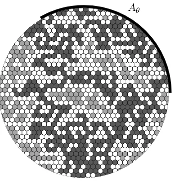
Fix some δ > 0, and consider site percolation with parameter p = 1/2 on the triangular grid of mesh δ. It is convenient to represent a percolation configuration by coloring the hexagonal faces of the dual grid, black for open, white for closed. LetBδ denote the union of all the black hexagons, and let Qδ(θ) denote the union ofAθ with all the connected components ofBδ∩U which meet Aθ. See Figure 1. Let Q(θ) denote a random subset of U whose law is the weak limit asδ ↓0 of the law ofQδ(θ). (The law ofQδ(θ) can be thought of as a probability measure
on the Hausdorff space of compact subsets ofU.) By [22, 23], the limit exists, and, moreover, it can be explicitly described via SLE6, as follows.
Recall from [22] that the limit ˜γ asδ↓0 of the outer boundary ofQδ(θ) consists ofAθ
concate-nated with the path of chordal SLE6 joining the endpoints ofAθ. By [22, 23], the scaling limit
of percolation is conformally invariant. Hence, it is not too hard to verify thatQ(θ) is obtained by “filling in” each component of U \γ˜ with an independent copy of Q(2π). A more precise statement is the following.
Theorem 2.1 (Smirnov). Letθ∈(0,2π), letγch denote the path of chordalSLE6 from1 toeiθ
inU, and let γ˜ denote the curve obtained by concatenating Aθ, clockwise oriented, with γch. Let W denote the collection of all connected components W of U\γ˜ such thatγ˜ has winding number −1about points inW. For eachW ∈ W, letψW :U →W be a conformal homeomorphism, and let QW denote an independent copy of Q(2π). Then the distribution of Q(θ) is the same as the distribution of
[
W∈W
ψW(QW).
Aθ
Figure 1: The set Qδ(θ).
Theorem 2.1 follows from the results and methods of [22]. See [23] for further details.
We are interested in the distribution of the distance from Q(θ) to 0. However, it is more convenient to study the distribution of a very closely related quantity, the conformal radius. Let U(θ) denote the component of 0 in U \Q(θ). (It follows from Theorem 2.1 or from the Russo-Seymour-Welsh Theorem that 0∈/ Q(θ) a.s.) Let ψ =ψθ :U(θ) → U be the conformal map, normalized by ψ(0) = 0 and ψ′(0) >0. Define the conformal radius r(θ) of U(θ) about 0 by r(θ) := 1/ψ
′(0). A well known consequence of the Koebe 1/4 Theorem and the Schwarz Lemma (see, e.g., [1]) is that
r(θ)
4 ≤dist 0, Q(θ)
≤r(θ), (2.1)
and therefore information about the distribution of r(θ) translates to information about the distribution of dist 0, Q(θ)
. Set
h(θ, t) :=P
r(θ)≤e
−t
. (2.2)
Note that fort >0,
h(0, t) = lim
θ↓0h(θ, t) = 0, (2.3)
follows from the Russo-Seymour-Welsh Theorem and the observation thatr(θ) tends to 1 if the diameter of Q(θ) tends to zero.
Lemma 2.2. In the range θ∈(0,2π), t >0, the functionh satisfies the PDE
κ 2∂
2
θh(θ, t) + cot
θ 2
∂θh(θ, t)−∂th(θ, t) = 0, (2.4)
withκ= 6.
Proof. We assume that γch and Q(θ) are coupled as in Theorem 2.1. Let Tch =Tch(θ) be the first timetsuch thatγch[0, t] disconnects 0 fromeiθ inU. Letγra denote the path of radial SLE6 from 1 to 0 inU, and letT =Tra(θ) denote the first time tsuch thatγra[0, t] disconnects 0 from
eiθ inU. From [13, Theorem 4.1] we know that up to time reparameterization, the restriction of
γra to [0, T] has the same distribution as the restriction of γch to [0, Tch]. We therefore assume that indeedγra restricted to [0, T] is a reparameterization ofγch restricted to [0, Tch]. Let Utbe
the connected component of U\γra[0, t] which contains 0, and let
gt:Ut→U
be the conformal map, normalized bygt(0) = 0, g′t(0)>0. By the definition of radial SLE6, the maps gt satisfy
∂tgt(z) =−gt(z)gt(z) +e i√κBt
gt(z)−ei
√
κBt , g0(z) =z , (2.5)
where κ = 6 andBt is Brownian motion on R with B0 = 0. Differentiating (2.5) with respect to z at z= 0 gives
g′t(0) =et. (2.6)
At timeT,γra separates 0 fromeiθ. Let W′ be the connected component ofU\γra[0, T] which contains 0. We distinguish between two possibilities. Either the boundary ofW′ onγra is on the right hand side of γra, in which case set ν := 1, or on the left hand side, and then set ν :=−1. In the notation of Theorem 2.1, if ν =−1, then W′ ∈ W/ . Hence, by (2.6) and the coupling of γra withQ(θ),
r(θ) =e
−T , ifν =−1. (2.7)
We also want to understand the distribution ofr(θ) givenγra andν = 1. In that case,W′ ∈ W. In Theorem 2.1, we may take the map ψW′ to satisfy ψW′(0) = 0. Let r′ denote the conformal radius about 0 ofU\Q
W′
, whereQW′ is as in Theorem 2.1. Thenr′ has the same distribution as
r(2π) and is independent from
S
s>0Fs, whereFs denotes theσ-field generated by (Bt:t≤s).
Moreover, by the chain rule for the derivative at zero,
r(θ) =r
′e−T, ifν = 1. (2.8)
To make use of the relations (2.7) and (2.8), we have to understand the relation betweenν and
FT. Recall thatgt γra(t)
= exp(i√κBt). Set fort < T,
Yt=Ytθ :=−iloggt(eiθ)−√κ Bt, (2.9)
withYθ
0 =θ and the log branch chosen continuously. That is,Yt is the length of the arc on∂U which corresponds under gt−1 to the union of Aθ with the right hand side γrhs[0, t] of γra[0, t]. Suppose, for a moment that ν = 1. That means that the boundary ofW′ is contained in γrhs and Aθ. Consequently, as t ↑ T, the harmonic measure from 0 of Aθ ∪γrhs tends to 1. By conformal invariance of harmonic measure, this means thatYt→2π ast↑T on the eventν= 1.
Similarly, we haveYt→0 ast↑T on the event ν=−1. SetYT := limt↑T Yt. By (2.7) and (2.8),
we now have
Phr(θ)≤e
−t FT
i
= 1{YT=2π}P
r′ ≤eT−t FT
Taking expectation gives
h(θ, t) =E
h(YTθ, t−T)
, (2.10)
where we use the fact that h(θ, t) = 1 fort≤0 and θ∈[0,2π]. From (2.5) and (2.9) we get
dYt= cot(Yt/2)dt−√κ dBt. (2.11)
By (2.10), for every constant s > 0 the process t 7→ h(Ytθ, s−t) is a local martingale on t <min{T, s}. The theory of diffusion processes and (2.10), (2.11) imply thath(θ, t) is smooth in the rangeθ∈(0,2π), t >0. By Itˆo’s formula at timet= 0
dh(Yt, s−t) =
κ
2∂ 2
θh(θ, s) + cot
θ
2 ∂θh(θ, s)−∂sh(θ, s)
dt−√κ ∂θh(θ, s)dBt.
Since h(Yt, s−t) is a local martingale, thedt term must vanish, and we obtain (2.4).
In order to derive boundary conditions, it turns out that it is more convenient to work with the following modified version ofh:
˜
h(θ, t) :=
Z 1
0
h(θ, t+s)ds .
Since,h is smooth, ˜h also satisfies the PDE (2.4).
Lemma 2.3. For every fixed t >0, the one sided θ-derivative of ˜h at 2π is zero; that is,
lim
θ↑2π
˜
h(2π, t)−˜h(θ, t)
2π−θ = 0. (2.12)
Proof. Letǫ >0 be very small and setθ= 2π−ǫ. Letδ >0 be smaller thanǫ, and letZ(r, ǫ) denote the event that there is a connected component of Bδ∩U which does not intersect Aθ but does intersect the two circles of radiiǫand r about the point 1.
We claim that there are constants c, α >0 such that
P
Z(r, ǫ)
≤c(ǫ/r)1+α, (2.13)
provided 0< δ < ǫ < r <2. This well known result is also used in Smirnov’s arguments. As we could not track down an explicit proof of this statement in the literature and for the reader’s convenience, we include a proof of this fact in the appendix.
LetQ′ :=Q(2π)\Q(θ). By letting δ ↓0, it follows from (2.13) that
P
diamQ′ ≥r
≤c(ǫ/r)1+α. (2.14)
It is easy to verify that there is a constantc1 >0 such that for every connected compactK ⊂U which intersects∂U, the harmonic measureµ(U, K,0) inU ofK from 0 satisfies
c−11 diamK≤µ(U, K,0)≤c1 diamK . (2.15)
Moreover, ifr(K) denotes the conformal radius ofU\K, then
minn−logr(K),1
o
≤c2 diamK
2
wherec2 is some constant. To justify this, note thatr(K) is monotone non-increasing in K and hence r(K) ≥r(B), whereB is the smallest disk with∂B orthogonal to∂U which contains K. For such aB, one can calculate r(B) explicitly, since the normalized conformal map fromU\B to U is conjugate to the mapz→
(The equality is due to conformal invariance of harmonic measure.) Combining this with (2.14) gives
Proof of Theorem 1.2. We are going to give a non-probabilistic proof based on the PDE and boundary conditions that we derived (but other justifications are also possible). Let Λ denote the differential operator on the left hand side of (2.4), and setS= (0,2π)×(0,∞). Set show that there are positive constantsc, c′ such that
∀t≥1, ∀θ∈[0,2π], c H(θ, t)≤˜h(θ, t)≤c′H(θ, t). (2.17)
But the definition of Λ shows that this contradicts ΛF <0. ThereforeF ≥0 on S∗. Sinceǫ >0 was arbitrary, this proves thatG≥0.
Now, note that Λ(2−2t−θ2)<0 for θ∈(0, π). Let
F1:=c1H−h˜+ 2−2t−θ2, F2 :=c2˜h−H+ 2−2t−θ2,
where the constantsc1, c2are chosen so thatF1 >0 andF2>0 on{π}×[0,1] and on [0, π]×{0}. The above argument applied to the functions Fj withS replaced by (0, π)×(0,1), shows that
c1H(θ,1) −˜h(θ,1) ≥ F1(θ,1) ≥ 0 and c2h˜(θ,1)−H(θ,1) ≥ F2(θ,1) ≥ 0 for θ ∈ [0, π]. By changing the constants c1 and c2 if necessary, we may make sure that this same inequalities hold for allθ∈[0,2π]. Yet another application of the same Maximum Principle argument, this time in the range [0,2π]×[1,∞) proves thatc1H−˜h ≥0 and c2˜h−H ≥0 for t≥1, thereby establishing (2.17).
The theorem now follows from (2.17), the definition of ˜h and (2.1).
3
The discrete exponent
We now show that the discrete exponent and the continuous exponent we derived are the same. The proof is quite direct. However, for exponents related to crossings of several colors (that is, black and white or occupied and vacant), the analogous equivalence is not as easy. See [24] for a treatment of this more involved situation.
Proof of Theorem 1.1. Letu(r) denote the probability thatQ=Q(2π) intersects the circle r∂U, and letC(R1, R2) denote the event that in site percolation with parameter p= 1/2 on the standard triangular grid, there is an open cluster crossing the annulus with radii R1 and R2 about 0. Let A(R) denote the event that there is an open path separating the circles of radii R and 2R about 0. By the definition of the scaling limit it follows that for all fixed r ∈ (0,1) there is somes0=s0(r) such that
∀R≥s0, u(r/2)/2≤P
C(rR, R)
≤2u(2r). (3.1)
LetRbe large,r >0 small, set ˜r= 2r, and letN be the minimal integer satisfyings0(r) ˜r−N > R. Note that the event {0↔CR}that 0 is connected to the circle CR satisfies
{0↔CR} ⊃ {0↔C2s0} ∩
N−1
\
j=0
C(s0r˜−j,2s0r˜−j−1)∩ A(s0r˜−j)
.
By the Harris/Fortuin-Kasteleyn-Ginibre (FKG) inequality, we therefore have
P[0↔CR]≥P[0↔C2s0]
N−1
Y
j=0 P
C(s0r˜−j,2s0r˜−j−1)
N−1
Y
j=0 P
A(s0r˜−j).
By the Russo-Seymour-Welsh Theorem (RSW), there is a constantc1 >0 such thatP
A(R)
≥
c1 for every R. Applying this and (3.1) in the above, gives
P[0↔CR]≥P[0↔C2s0]c
N
1 u(r/2)/2
N
By Theorem 1.2, logu(r)/logr →5/48 asr↓0. Therefore,
is similar (using independence on disjoint sets, in place of FKG), and is left to the reader.
4
Counterclockwise loops for
SLE
κProof of Theorem 1.3. Let κ > 4, κ 6= 8. Let γ denote the path of radial SLEκ started
from 1, and for θ∈[0,2π] letγθt denote the concatenation of the counterclockwise oriented arc ∂U\Aθ with γ[0, t]. Let E(θ, t) denote the event that γ
We now need to verify that ˆh also satisfies the Neumann boundary condition (2.12). It is immediate that there is a constantc1 >0 such that
∀t >0, ∀θ∈[π/2,3π/2],
Observe from (2.11) that
∂t Ytθ2 −Yθ
1
t
≤0. Therefore, onS we have Yθ2
τ −Yτθ1 ≤θ2−θ1. Hence, by (4.1) combined with (4.2), ˆ
h(θ2, t1)−ˆh(θ1, t1)≤c1P[S] (θ2−θ1). (4.3) But whenθ1< θ2 ≤2π are both close to 2π, we know that with probability close to 1 there will be some timet0 ∈(0, t1) such thatYtθ01 = 2π. In that case also Y
θ2
t0 = 2π, and henceY
θ1
t =Ytθ2
for all t∈[t0,Tˆ). In particular, P[S]→0 as θ1→2π. By (4.3) we get the Neumann condition: lim
θ↑2π∂θ
ˆ
h(θ, t1) = 0.
Now the proof of the theorem is completed exactly as for the corresponding proof of (2.17).
A
Appendix: an a priori half plane exponent
We now give a brief outline of the proof of the a priori estimate (2.13) on the probability that there exists three disjoint crossings of a half-annulus. This is based on the exponent for the existence of two disjoint crossings.
Lemma A.1. There is a constant c >0 such that for allR > r >2 the probability f(R, r) that there are two disjoint crossings between CR and Cr within the half-plane iH =
z: Rez≤0} in site percolation with parameter p= 1/2 on the standard triangular grid satisfies
c−1r/R ≤f(R, r)≤c r/R .
Loosely speaking, this lemma says that the two-arms half plane exponent is 1. Note that the half-plane exponents for SLE6 were calculated in [12, 14]. They are now valid for critical site percolation on the triangular grid, since SLE6 describes the scaling limit. However, to show the equivalence, this lemma seems to be needed.
Proof. LetSR be the strip SR := z ∈C : Rez ∈[−R,0] , and let XR be the set of clusters inSR which join the intervalIR := [−iR, iR]⊂iR to the line LR:= −R+iR. It follows from RSW that
sup
R>0 E
|XR|
<∞, inf
R>2P
|XR|>2
>0. (A.1)
Define the eventDR that there exists a path of occupied site inSRjoining the origin toLR and
a path of vacant sites in SR joining the vertex directly below the origin to LR. Note that DR
is the same as the event that there is some C∈XR such that 0 is the lowest vertex in C∩iR. By invariance under vertical translations, since the number of vertices inIR is of orderR, (A.1)
implies that
∀R >2, P[DR]≍1/R ,
whereg≍h means that g/his bounded and bounded away from zero.
from 0 toLR inSR, it follows thatP[DR] is equal to the probability of the event DR2 that there
are disjoint open paths inSR connecting the origin and the vertex below the origin to LR. Let C2
R be the event that there are two disjoint paths connecting the origin and the vertex below
the origin toCR in iH. Clearly, C
2
R ⊃ DR2. On the other hand, whenR is sufficiently large, by
RSW the probability that there are two disjoint left-right crossings of each of the the rectangles [−R,0]×[R/10, R/5] and [−R,0]×[−R/5,−R/10] is bounded away from zero. Therefore, the FKG inequality implies that there is some constantc >0 such that
P[D2
R]≥cP[C22R].
Consequently, we find thatP[C2
R]≍R−1 forR >2. Another application of RSW and FKG as
in the proof of Theorem 1.1 shows that
P[CR2]≍f(R, r)P[Cr2], when R >2r >4. The lemma follows.
By using RSW yet again combined with the van den Berg-Kesten inequality (BK), it follows that there are c, ǫ > 0 such that the probability that Cr and CR are connected in iH by two open crossings and one closed crossing is at most c(r/R)1+ǫ, when r > 1. This immediately implies (2.13), because the existence of a cluster inU intersectingCr andCǫ but not intersecting
Aθ implies that there are also two disjoint closed crossings fromCǫ to Cr inU.
By looking at the right-most vertices of clusters of diameter greater thanR, an argument similar to the proof of Lemma A.1 can be used to prove directly that the three-arms exponent in a half-plane is 2. An analogous argument [8, Lemma 5] shows that the multicolor five-arms exponent in the plane is equal to 2, which then implies that the multicolor six arms exponent is strictly larger than 2. (This is also an instrumental a priori estimate in [23].) Similarly, the Brownian intersection exponentξ(2,1) = 2 can be easily determined [9], and a direct proof also works for some exponents associated to loop-erased random walks (e.g., [10]). However, these exponents that take the value 1 or 2 are exceptional. For the determination of fractional exponents, such as, for instance, the one-arm exponent in the present paper, such direct arguments do not work.
B
The monochromatic 2-arm exponent
This informal appendix will discuss the monochromatic 2-arm exponent (sometimes also called “backbone exponent”); that is, the exponent describing the decay of the probability that there are two disjoint open crossings from Cr to CR. So far, despite some attempts, there is no
established prediction in the theoretical physics community for the value of this exponent, as far as we are aware. Simulations [4] show that its numerical value is.3568±.0008.
and the multichromatic k-arm exponent. The multichromatic exponents withk≥2 can all be worked out from [13] combined with [22] (see [24]). We now show (ommiting many details) that the monochromatic 2-arm exponent is in fact also the leading eigenvalue of a differential operator. So far, we have not been able to solve explicitely the PDE problem and to give an explicit formula for the value of the exponent, but this might perhaps be doable by someone more proficient in this field.
Like in the one-arm case, we have to work with a slightly more general problem. Let α, β >0 satisfy α +β < 2π, and let A and A′ be two consecutive arcs on ∂U with lengths α and β, respectively, and setA′′=∂U\(A∪A
′). Letγ = 2π−α−β denote the length ofA′′ and letQ be the scaling limit of the set of points p∈U which are connected toA′′ by two paths lying in the union ofA′with the set of black hexagons, such that the two paths do not share any hexagon except for the hexagon containingp. LetG(α, γ, t) be the probability that the conformal radius of U\Q about 0 is at most e
−t. Using arguments as above, it is easy to check, by starting an
SLE6 path from the common endpoint ofA and A′, that G(α, γ, t) satisfies the PDE
3∂α2G+ cot α 2
∂αG+
cot α+γ 2
−cot α 2
∂γG−∂tG= 0.
The Dirichlet condition
G= 0, when γ= 0
is immediate. Similarly, one can check that for all γ 6= 0,
G(0, γ) =G(0,2π).
Finally, using arguments as for the one-arm exponent, one can show that the boundary condition on α+γ = 2π is
∂γG= 0.
Hence, the monochromatic two-arm exponent is a number (and in fact the unique number)λ >0 such that there is a non-negative functionG1(α, γ), not identically zero, such thate−λtG1(α, γ) solves the above PDE and has the corresponding boundary behaviour (one can fix the multi-plicative constant by settingG1(0,2π) = 1). We have been unable to guess an explicit solution to this boundary value problem. Some insight might be gained by noting that when α and γ go down to zero, the solution should behave like Cardy’s [3] formula in α/(α+γ), which is a hypergeometric function.
One can rewrite the PDE using other variables. In terms of the functionG2(α, β) :=G1(α,2π− α−β), one looks for the non-negative eigenfunctions of the more symmetric operator
3(∂2α−2∂α∂β+∂β2) + cot
α 2
∂α−cot
β 2
∂β
with boundary conditions (for α, β >0,α+β <2π),
References
[1] L.V. Ahlfors (1973), Conformal Invariants, Topics in Geometric Function Theory, McGraw-Hill,
New-York.
[2] M. Aizenman, B. Duplantier, A. Aharony (1999), Path crossing exponents and the external perimeter
in 2D percolation. Phys. Rev. Let.83, 1359–1362.
[3] J.L. Cardy (1992), Critical percolation in finite geometries, J. Phys. A,25L201–L206.
[4] P. Grassberger (1999), Conductivity exponent and backbone dimension in 2-d percolation, Physica
A 262, 251.
[5] G. Grimmett,Percolation, Springer, 1989.
[6] H. Kesten, Percolation Theory for Mathematicians, Birkha¨user, 1982.
[7] H. Kesten (1987), Scaling relations for 2D-percolation, Comm. Math. Phys.109, 109–156.
[8] H. Kesten, V. Sidoravicius, Y. Zhang (1998), Almost all words are seen in critical site percolation
on the tringular lattice, Electr. J. Prob.3, paper no. 10.
[9] G.F. Lawler,Intersection of Random Walks, Birkh¨auser, 1991.
[10] G.F. Lawler (1999), Loop-erased random walk,Perplexing Probability Problems: Festschrift in Honor
of Harry Kesten (M. Bramson and R. Durrett, eds), 197–217, Birkh¨auser, Boston.
[11] G.F. Lawler (2001), An introduction to the stochastic Loewner evolution, preprint.
[12] G.F. Lawler, O. Schramm, W. Werner (1999), Values of Brownian intersection exponents I: Half-plane exponents, Acta Mathematica, to appear.
[13] G.F. Lawler, O. Schramm, W. Werner (2000), Values of Brownian intersection exponents II: Plane exponents, Acta Mathematica, to appear.
[14] G.F. Lawler, O. Schramm, W. Werner (2000), Values of Brownian intersection exponents III: Two sided exponents, Ann. Inst. Henri Poincar´e, to appear.
[15] B. Nienhuis (1984), Coulomb gas description of 2-D critical behaviour, J. Stat. Phys.34, 731-761
[16] B. Nienhuis, E.K. Riedel, M. Schick (1980), Magnetic exponents of the two-dimensional q-states
Potts model, J. Phys A13, L. 189–192.
[17] M.P.M. den Nijs (1979), A relation between the temperature exponents of the eight-vertex and the q-state Potts model, J. Phys. A12, 1857–1868.
[18] D. Revuz, M. Yor,Continuous Martingales and Brownian Motion, Springer, 2nd Ed., 1994.
[19] S. Rohde, O. Schramm (2001), Basic properties of SLE, arXiv:math.PR/0106036.
[20] O. Schramm (2000), Scaling limits of loop-erased random walks and uniform spanning trees, Israel
J. Math. 118, 221–288.
[21] O. Schramm (2001), A percolation formula, Electronic Comm. Prob.6, paper no. 12, 115–120.
[22] S. Smirnov (2001), Critical percolation in the plane: Conformal invariance, Cardy’s formula, scaling
limits, C. R. Acad. Sci. Paris Sr. I Math.333no. 3, 239–244.
[23] S. Smirnov (2001), in preparation.