SPECTRUM LOCALIZATION OF REGULAR MATRIX POLYNOMIALS AND FUNCTIONS∗
A.G. MAZKO†
Abstract. This paper is devoted to the spectrum localization problem for regular matrix polynomials and functions. Sufficient conditions are proposed for spectrum placement in a wide class of regions bounded by analytical curves. These conditions generalize the known linear matrix inequalities (LMI) approaches to stability analysis and pole placement of polynomial matrices. In addition, a method of robust spectrum placement is developed in the form of the LMI systems for a parametric set of matrix polynomials.
Key words. Matrix polynomial, Eigenvalue, Spectrum localization, Linear matrix inequality, Robust stability.
AMS subject classifications.5A18, 15A22, 26C10.
1. Introduction. Many theoretical and applied problems are associated with the analysis of spectral properties of matrix functions including polynomial matrices. If direct evaluation of the eigenvalues does not leads to desirable outcomes, there are problems of their estimation and localization with respect to certain regions of a complex plane. Numerous works are devoted to solving these problems (see, e.g., [1]–[4]).
In this paper, we study the problem of spectrum localization for matrix poly-nomials and functions. We establish sufficient conditions for checking location of all eigenvalues of regular matrix functions in specified regions of the complex plane. The results obtained essential complement and generalize the known approaches to pole placement of polynomial matrices reduced to the LMI technics (see, e.g., [5] and [3, Section 2.7]). Moreover, we expand the obtained results to a parametric set of matrix polynomials in the form of the LMI systems.
Notation: ⊗, ∗, and T denote the matrix operations of the Kronecker pro-duct, complex conjugation and transposition, respectively; In is the identity n×n
matrix; On and Onm denote the zero n×n and n×m matrix, respectively; the
matrix inequalities X > Y,X ≥Y, and X Y mean that the matrix X−Y is
po-∗Received by the editors January 4, 2010. Accepted for publication May 28, 2010. Handling
Editor: Harm Bart.
†Institute of Mathematics, Ukrainian Academy of Sciences, Kyiv, Ukraine
sitive definite, positive semidefinite, and nonzero positive semidefinite, respectively; i(X) ={i+(X), i−(X), i0(X)}is the inertia of the Hermitian matrixX =X∗
consist-ing of its numbers of positive (i+(X)), negative (i−(X)), and zero (i0(X)) eigenvalues
(taking into account the multiplicities); λmax(X) (λmin(X)) is the maximum
(mini-mum) eigenvalue of the Hermitian matrixX.
2. Matrix function and analytical regions. Consider the regular matrix function
F(λ) =
m X
i=0
fi(λ)Ai, detF(λ)6≡0, λ∈C1,
(2.1)
where A0, . . . , Am ∈ Cn×n are n×n matrices. Let σ(F) be a spectrum of the
matrix function that consists of all eigenvalues. Suppose that the scalar functions f0(λ), . . . , fm(λ) are analytical in a neighbourhood ofσ(F) and let
zm(λ) = [f0(λ), . . . , fm(λ)]6= 0, λ∈σ(F).
We study a location of the spectrum with respect to regions in the complex plane of the type
Ω =λ∈C1: i+(V(λ, λ))≥1 , Ω =ˆ λ∈C1: V(λ, λ)≤0 ,
(2.2)
where V(λ, λ) is a Hermitian matrix-valued function. It is obvious that Ω∩Ω =ˆ ∅
and Ω∪Ω =ˆ C1.
Let’s introduce the block matrices
A=
A0
.. . Am
, G=
G0
.. . Gm
, L=
L00 · · · L0m
..
. . .. ...
Lm0 · · · Lmm
, W =
L G
G∗ H
.
HereAi, Gi, Lij, H are then×nblocks, and the matrices LandW are Hermitian.
We define the matrix A⊥ = [B
0, . . . , Bm]∗ of size n(m+ 1)×nmas a basis for
the right null space ofA∗. Then
A⊥∗A= 0, A+A=I
n, detT 6= 0, T = [A+∗, A⊥],
(2.3)
where A+ = (A∗A)−1A∗ is the pseudoinverse matrix. Under regularity condition of the matrix function F(λ), it is always possible to construct the matrix A⊥ with specified properties.
Let the regions (2.2) be defined by
V(λ, λ) =
m X
i,j=0
If
In(m+1), AWIn(m+1), A
∗ >0 (2.4)
or
A⊥∗LA⊥>0, (2.5)
thenσ(F)∩Ω =ˆ ∅, i.e. all the eigenvalues of F(λ)lie within Ω.
Proof. It is obvious thatF(λ) = Zm(λ)A and V(λ, λ) =Zm(λ)LZm∗(λ), where
Zm(λ) = [f0(λ)In, . . . , fm(λ)In] =zm(λ)⊗In. We multiply (2.4) on the left and on
the right byZm(λ) andZm∗(λ), respectively. Then we obtain
F(λ)G∗(λ) +G(λ)F∗(λ) +F(λ)HF∗(λ) +V(λ, λ)>0,
where G(λ) is a matrix function. Let v∗
0 6= 0 be the left eigenvector of the matrix
function F(λ) corresponding to an eigenvalue λ0 ∈ σ(F). Multiplying the matrix
inequality on the left and on the right byv∗
0 andv0, respectively, atλ=λ0, we have
v∗
0V(λ0, λ0)v0>0, that meansλ0∈Ω.
Let’s multiply the matrix inequality (2.4) on the left and on the right byT∗ and T, respectively, and use the known criterion of positive definiteness of a block matrix:
P N
N∗ Q
>0 ⇐⇒ Q >0, P > N Q−1N∗. (2.6)
In this case,
P =H+G∗A+∗+A+G+A+LA+∗, Q=A⊥∗LA⊥, N= (G∗+A+L)A⊥.
Since last inequality in (2.6) may be always satisfied by choosing H > 0, for inequality performance (2.4), it is enough to demand that Q > 0. Therefore, the inclusionσ(F)⊂Ω also follows from (2.5).
Note that, in Lemma 2.1, it is necessary to have the inequalities
n(m+ 1)≤i+(W)< n(m+ 2), 1≤i+(L)< n(m+ 1).
As H, there may be any positive definite matrix, for example, H = In. If the
inequality (2.4) holds forH≤0, then all the eigenvalues of the matrix functionG(λ) as well as theF(λ) should belong to Ω.
Theorem 2.2. If
AG∗+GA∗+AHA∗+ Γ⊗X >0, X0; (2.7)
or
m X
i,j=0
γijBiXB∗j >0, X 0;
(2.8)
then all the eigenvalues of the matrix function F(λ)lie within the region
Ω =nλ∈C1:f(λ, λ) =
m X
i,j=0
γijfi(λ)fi(λ)>0 o
.
Letf0(λ)6= 0 in a neighbourhood ofσ(F), and let regions Ω and ˆΩ be defined as
in (2.2) with
V(λ, λ) =
"
Ψ∗(λ)LΨ(λ) f
0(λ)Ψ∗(λ)G
f0(λ)G∗Ψ(λ) f0(λ)f0(λ)H #
,Ψ(λ) =
−f1(λ)In · · · −fm(λ)In
f0(λ)In · · · On
..
. . .. ...
On · · · f0(λ)In
.
Lemma 2.3. If
[A∗, I
n]W[A∗, In]∗>0,
(2.9)
thenσ(F)∩Ω =ˆ ∅, i.e. all the eigenvalues of F(λ)lie within Ω.
Proof. Let v0 6= 0 be the right eigenvector of the matrix function F(λ)
corre-sponding to an eigenvalueλ0∈σ(F). Multiplying (2.9) on the left and on the right
byf0(λ0)v∗0 andf0(λ0)v0, respectively, and taking into account the relations
f0(λ0)A0v0=− m X
i=1
fi(λ0)Aiv0, w∗0 = [v0∗A∗1, . . . , v∗0A∗m, v0∗]6= 0,
we havew∗
0V(λ0, λ0)w0>0, that meansλ0∈Ω.
Note that, in Lemma 2.3, it is necessary the inequalityn≤i+(W)< n(m+ 2).
Theorem 2.4. If
m X
i,j=0
γijA∗iXAj>0, X0,
then all the eigenvalues of the matrix function F(λ)lie within the region
Ω =λ∈C1: i+(U(λ, λ))≥1 ,
where
U(λ, λ) = Φ∗(λ)ΓΦ(λ), Φ(λ) =
−z(λ) f0(λ)Im
, z(λ) = [f1(λ), . . . , fm(λ)].
Theorem 2.4 follows from Lemma 2.3 whenGand H are zero, andL= Γ⊗X. Similar statement was formulated in [2] under weaker restrictions (controllability type) to the matrix expressions in (2.10). Lemmas 2.1 and 2.3 develop and complement the known approaches to pole placement of matrix functions (see [2, pp. 94–98] and [3, Section 2.7]) by means of the LMI (2.4), (2.5), (2.9) and their special cases (2.7), (2.8) and (2.10).
Remark 2.5. If we choose Γ in the form
Γ =
0 1 O1m−1
1 q O1m−1
Om−1 1 Om−1 1 −Q−1
, Q=Q∗>0,
then Ω in Theorem 2.4 can be described by the scalar function:
Ω =nλ∈C1:f(λ, λ) =zm(λ)eΓzm∗(λ)>0o, Γ =e
q −1 O1m−1
−1 0 O1m−1
Om−1 1 Om−1 1 Q .
Example 2.6. Consider the regular matrix quasipolynomial
F(λ) =A0+λA1+e−λτ1A2+· · ·+e−λτm−1A
m, τi≥0, i= 1, m−1.
If any numbersq,q1>0, . . . , qm−1>0 and matrixX 0 satisfy the matrix inequality
A∗0XA1+A∗1XA0+qA∗1XA1− mX−1
i=1
1 qi
A∗i+1XAi+1>0,
(2.11)
then according to Theorem 2.4 all the eigenvalues ofF(λ) lie within the region
Ω =nλ∈C1: λ+λ < q+
mX−1
i=1
qie−(λ+λ)τi o
.
If q ≤ −q1− · · · −qm−1, then given region is located in the left half-plane. In this
3. Matrix polynomial and algebraic regions. Given the regular matrix polynomial of sizen×nand degrees
F(λ) =A0+λA1+· · ·+λsAs, detF(λ)6≡0, λ∈C1,
(3.1)
we consider the class of algebraic regions:
Λk = n
λ∈C1: f(λ, λ) =
k X
i,j=0
γijλiλ j
>0o, (3.2)
where γij are entries of the Hermitian matrix Γ, ands≥1,k≥1. We assume that
Λk 6=∅and Λk6=C1, i.e. i±(Γ)6= 0.
It is obvious that any region Λ1 is bounded by a line or a circle. In particular,
the matrices
Γ =
0 −1
−1 0
, Γ =
1 0
0 −1
, (3.3)
correspond to the left half-plane and the unit disk. The class Λ2 contains all the
regions bounded by algebraic curves of the second order.
Letm= max{s, k}and r=m−k. We construct the block matrices
A=
A0
.. . Am
, G=
G0
.. . Gm
, X =
X00 · · · X0r
..
. . .. ...
Xr0 · · · Xrr
,
of sizesn(m+ 1)×n,n(m+ 1)×nandn(r+ 1)×n(r+ 1), respectively, and introduce the linear operators
L(X) =C(Γ⊗X)CT, M(X) =D(Γ⊗X)D∗, (3.4)
where
C=R⊗In= [C0, . . . , Ck], D=A⊥∗C= [D0, . . . , Dk],
R=E,∆E, . . . ,∆kE, ∆ =
O1m 0
Im Om1
, E=
Ir+1
Ok r+1
,
A⊥∗= [B
0, . . . , Bm] is the matrix defined by (2.3). In the case ofk > s, the blocksAi
(i > s) should be chosen in such a way that the spectrum of the matrix polynomial
Fm(λ) =A0+λA1+· · ·+λmAm containsσ(F). For example, we can suppose that
Let ˆΛk , \Λk be the closed complement of Λk, and let Λr(X) be the closed
region defined by the block Hermitian matrixX:
Λr(X) = n
λ∈C1: Zr(λ)XZr∗(λ) =
r X
i,j=0
λiλjXij≥0 o
, Zr(λ) = [In, λIn, . . . , λrIn].
Theorem 3.1. Let for some matricesG,H =H∗,X =X∗, the inclusion
ˆ
Λk⊆Λr(X)
(3.5)
and one of the matrix inequalities
AG∗+GA∗+AHA∗+L(X)>0 (3.6)
or
M(X)>0 (3.7)
hold. Then all the eigenvalues of the matrix polynomial F(λ) lie within the region
Λk.
Proof. The matrixRof size (m+ 1)×(k+ 1)(r+ 1) has the following structure:
R=E,∆E, . . . ,∆kE=
Ir+1
O1r+1
Ok−1r+1
O1r+1
Ir+1
Ok−1r+1
· · ·
O1r+1
Ok−1r+1
Ir+1 .
It is obvious that
Fm(λ) =Zm(λ)A, f(λ, λ) =zk(λ)Γzk∗(λ),
whereZm(λ) =zm(λ)⊗In,zm(λ) = [1, λ, . . . , λm]. Using the structure of matrixC
and the Kronecker products properties, we have
Zm(λ)C= (zm(λ)⊗In)(R⊗In) =zm(λ)R⊗In =
= [zr(λ), λzr(λ), . . . , λkzr(λ)]⊗In=zk(λ)⊗zr(λ)⊗In=zk(λ)⊗Zr(λ).
Multiplying (3.6) on the left and on the right by the full rank matrices Zm(λ)
andZ∗
m(λ), respectively, we obtain
Fm(λ)G∗m(λ)+Gm(λ)Fm∗(λ)+Fm(λ)HFm∗(λ)+ [zk(λ)⊗Zr(λ)](Γ⊗X)[zk∗(λ)⊗Zr∗(λ)] =
whereGm(λ) =G0+λG1+· · ·+λmGm is a matrix polynomial.
Let λ = λ0 ∈ σ(F) be an arbitrary eigenvalue of F(λ). Also we assume that
λ06∈Λk, i.e. λ0∈Λˆk. Then, according to (3.5),f(λ0, λ0)Zr(λ0)XZr∗(λ0)≤0. Thus,
Fm(λ0)G∗m(λ0) +Gm(λ0)Fm∗(λ0) +Fm(λ0)HFm∗(λ0)>0.
However, this is not true, becauseσ(F)⊆σ(Fm) and
v∗
0[Fm(λ0)G∗m(λ0) +Gm(λ0)Fm∗(λ0) +Fm(λ0)HFm∗(λ0)]v0= 0,
where v∗
0 6= 0 is the left eigenvector of the matrix polynomial Fm(λ) corresponding
to λ0 ∈σ(Fm). From this contradiction, it follows that, under conditions (3.5) and
(3.6), it should beλ0∈Λk.
From (3.5) and (3.7), it also follows thatσ(F)⊂Ω. It is established by multi-plying (3.6) on the left and on the right byT andT∗, respectively, and applying the criterion (2.6) (see the proof of Lemma 2.1).
Theorem 3.1 develops known approach for the spectrum localization of a matrix polynomial proposed in [5] for the class of regions Λ1. We do not use any restrictions
to the order of the algebraic curves. In addition, condition (3.5) generally does not demand the positive definiteness of solutions of the corresponding matrix inequalities. The results obtained in [4] extend the approach of [5] by considering algebraic regions
Ddescribed by the quadratic matrix inequalities and involving the optimization algo-rithms. Every D-region can always be written as a finite set of Ω-regions. However, the converse procedure is nontrivial and unsolved problem for the present.
Remark 3.2. The proof of Theorem 3.1 can be obtained as a corollary of Lemma 2.1. Indeed, in the case of the matrix polynomial, we suppose thatfi(λ) =λi fori=
0, m, and, in virtue of (3.5), Ω⊆Λk. The restriction (3.5) holds for arbitrary region
Λk when Λr(X) = C1. For example, we can find X as an algebraically nonnegative
defined matrix, in particular, nonnegative defined matrix in usual sense.
Definition 3.3. The block Hermitian matrixX is called algebraically positive
(nonnegative) defined if
Zr(λ)XZr∗(λ) = r X
i,j=0
λiλjX
ij >0 (≥0), ∀λ∈C1.
Note that all the matrices of the type
X =
Xp On(p+1)n(r−p)
On(r−p)n(p+1) On(r−p)n(r−p)
, Xp=
X00 · · · X0p
..
. . .. ...
Xp0 · · · Xpp
are algebraically positive defined. These matrices are positive defined whenp=r.
Remark 3.4. If k ≥s, then m =k, r = 0, and C = In(k+1). In this case, in
(3.6) and (3.7), we suppose L(X) = Γ⊗X andM(X) =A⊥∗L(X)A⊥. In addition, in Theorem 3.1, we use the inequalityX=X∗0 instead of (3.5).
Remark 3.5. Under certain restrictions, the proposed sufficient conditions for spectrum inclusion σ(F) ⊂ Λk can become necessary conditions. If the LMI (3.6)
holds, theni+(L(X))≥nm, and consequently (see [3, Theorem 4.2.1]),
i+(Γ)i+(X) +i−(Γ)i−(X)≥nm.
This inequality is necessary also for feasibility of the LMI (3.7). Particularly, in the case of k ≥ s and X > 0, it is necessary that i(Γ) = {k,1,0}. The necessary and sufficient solvability conditions of (3.7) can be studied via the general theorems on inertia of Hermitian solutions of transformable matrix equations [2, 3]. Especially, such conditions are connected with constraints for the inertiai(Γ) and the property of simultaneous reducibility of the matrix coefficients Di = A⊥∗Ci (i = 0, k) to
triangular form through common similarity transformation. Whenk= 1, the matrices Di are quadratic (see, e.g., Theorem 3.7 and Example 3.8 below).
Notice that if detA06= 0, then in (2.3),A⊥∗ always can be chosen as
A⊥∗ =
ˆ
A1 In · · · On
..
. ... . .. ... ˆ
Am On · · · In
, Aˆi =
−AiA−01, i≤s,
On, i > s.
(3.8)
Whenk=s, the operatorM(X) in (3.7), in virtue of (3.8), has the block structure:
M(X) =
Y11(Z) · · · Y1s(Z)
..
. . .. ...
Ys1(Z) · · · Yss(Z)
, X=A0ZA∗0,
(3.9)
whereYpq(Z) =γ00ApZA∗q −γp0A0ZA∗q−γ0qApZA∗0+γpqA0ZA∗0, p, q= 1, s.
If detA0= 0, then we consider, instead of F(λ) and Λk, the matrix polynomial
and region, respectively, as follows:
Fα(λ) =F(λ+α) = s X
i=0
λiA
αi, Λαk = n
λ∈C1:f(λ+α, λ+α) =
k X
i,j=0
γα ijλ
iλj>0o,
where Aα0 = F(α), detAα0 6= 0. Since F(λ) is a regular matrix polynomial, there
is α 6∈ σ(F) with specified properties. Thus, σ(F) ⊂ Λk ⇐⇒ σ(Fα) ⊂ Λαk, and
There are various methods of reduction of spectral problems for matrix polyno-mials to similar problems for linear pencils of matrices (see, for example, [6]–[9]). We use the method [9] based on applying the matrices of type A⊥ satisfying (2.3). Using the block representationA⊥∗ = [B
0, . . . , Bs], we construct the linear pencil of
matrices
D1−λD0= [B1, . . . , Bs]−λ[B0, . . . , Bs−1]
(3.10)
and consider the following relations
v∗F(λ) = 0, v6= 0; (3.11)
u∗(D1−λD0) = 0, u6= 0;
(3.12)
u∗A⊥∗=v∗Z
s(λ), v=B0∗u6= 0.
(3.13)
The relations (3.11) and (3.12) define the eigenvalues and the corresponding left eigenvectors of matrix polynomial (3.1) and pencil (3.10), respectively.
It is easy to establish equivalence of (3.12) and (3.13). On the other hand, from definition ofA⊥ and representations F(λ) =Z
s(λ)A, it follows that (3.11) is
equiv-alent to (3.13) for certain vector u 6= 0. Hence, (3.11) and (3.12) are equivalent. Additionally, identical fulfilment of one of equalities (3.11) or (3.12) at everyλ∈C1
implies identical fulfilment of other of them. This means that regularity properties of matrix polynomial (3.1) and pencil (3.10) are equivalent, too.
Lemma 3.6. Sets of all the various eigenvalues λi of matrix polynomial (3.1)
and pencil (3.10) coincide, and their corresponding left eigenvectors are related by
v∗
i =u∗iB0 (i= 1, l).
Now we formulate criteria of inclusionσ(F)⊂Λ1. In this case,
E=
Is
O1s
, ∆ =
O1s 0
Is Os1
,
M(X) =γ00D0XD∗0+γ01D0XD1∗+γ10D1XD∗0+γ11D1XD∗1,
(3.14)
where D0 and D1 are matrices defined in (3.10). In particular, for matrix (3.8), we
have
D0=
ˆ
A1 In · · · On
..
. ... . .. ... ˆ
As−1 On · · · In
ˆ
As On · · · On
Considering Lemma 3.6 and general properties of positive invertible operators in the space of the Hermitian matrices, it is possible to formulate the following statement (see [2, 3]).
Theorem 3.7. The inclusionσ(F)⊂Λ1holds if and only if there exist Hermitian
matricesX andY satisfying the relations
(a) M(X) =Y ≥0, D0XD0∗≥0, rank [D1−λD0, Y]≡ns (λ∈Λˆ1).
If D0 is nonsingular, then(a) is equivalent to each of the following statements:
(b)the matrix inequality M(X)>0 has a solutionX >0;
(c) given anyY >0, the matrix equationM(X) =Y has a solutionX >0;
(d) operator M is positive invertible with respect to a cone of nonnegative definite matrices.
The proof of sufficiency of the criterion (a) consists in the following. If we assume that some eigenvalue λ ∈ Λˆ1, then, according to (3.12), for the corresponding left
eigenvectoru∗, the inconsistent relations should be held true:
f(λ, λ)≤0, u∗D
0XD0∗u≥0, f(λ, λ)u∗D0XD0∗u=u∗Y u >0.
Provided that σ(F)⊂Λ1, the matrices X andY in criterion (a) always can be
constructed in the form [2]
X=ZXZˆ ∗, Y =D0ZY Zˆ ∗D∗0, rank[D1Z, D0Z] = rank(D0Z).
This fact is established using the Kronecker canonical form of a regular matrix pencil [11]. IfD0is nonsingular, then the criteria (b), (c) and (d) follow from known theorems
on localization of eigenvalues by means of the generalized Lyapunov equation.
Example 3.8. LetF(λ) =A0+λA1be a regular pencil ofn×nmatrices, and Λ1 be a region of the form (3.2). The matrix inequality (3.6) in Theorem 3.1 may be
expressed as
A0HA∗0+A0G0∗+G0A∗0+γ00X A0HA∗1+A0G∗1+G0A∗1+γ01X
A1HA∗0+A1G0∗+G1A∗0+γ10X A1HA∗1+A1G∗1+G1A∗1+γ11X
>0.
The matrix inequality (3.7) constructed for the linear pencil Fα(λ) = F(α) +λA1
and the regions Λα
1 ={λ∈C1:f(λ+α, λ+α)>0}in virtue of A⊥∗ = [B0, B1] =
[−A1F−1(α), In] is reduced to the form
M(X) =γ00A1ZA∗1−γ10A0ZA∗1−γ01A1ZA∗0+γ11A0ZA∗0>0,
matrix pencil F(λ) and regions Λ1. In particular, existence of solutions Z=Z∗>0
of the matrix inequalities
A0ZA∗1+A1ZA∗0>0, A1ZA∗1−A0ZA∗0>0
is equivalent to location of the spectrumσ(F) inside the left half-plane and the unit disk, respectively.
Example 3.9. Let F(λ) = A0+λA1+λ2A2 be a quadratic pencil of n×n matrices, and Λk be a region of the type (3.2) for k ≤ 2. Then the expression
AG∗+GA∗+AHA∗ in (3.6) has the block form
A0G∗0+G0A∗0+A0HA∗0 A0G∗1+G0A∗1+A0HA∗1 A0G2∗+G0A∗2+A0HA∗2
A1G∗0+G1A∗0+A1HA∗0 A1G∗1+G1A∗1+A1HA∗1 A1G2∗+G1A∗2+A1HA∗2
A2G∗0+G2A∗0+A2HA∗0 A2G∗1+G2A∗1+A2HA∗1 A2G2∗+G2A∗2+A2HA∗2 .
For the class of regions Λ1, we have 1 =k < s= 2,m= 2,r= 1,
E=
1 0 0 1 0 0
, ∆ =
0 0 0
1 0 0
0 1 0
, R=
1 0 0 0
0 1 1 0
0 0 0 1
, X =
X00 X01
X10 X11
,
L(X) =
γ00X00 γ00X01+γ01X00 γ01X01
γ00X10+γ10X00 1 P i,j=0
γijX1−i1−j γ01X11+γ11X01
γ10X10 γ10X11+γ11X10 γ11X11 .
For the class of regions Λ2, in (3.6) and (3.9), we use the operators
L(X) =
γ00X γ01X γ02X
γ10X γ11X γ12X
γ20X γ21X γ22X
, M(X) =
Y11(Z) Y12(Z)
Y21(Z) Y22(Z)
,
where
Y11(Z) =γ00A1ZA∗1−γ10A0ZA∗1−γ01A1ZA∗0+γ11A0ZA∗0,
Y12(Z) =γ00A1ZA∗2−γ10A0ZA∗2−γ02A1ZA∗0+γ12A0ZA∗0,
Y22(Z) =γ00A2ZA∗2−γ20A0ZA∗2−γ02A2ZA∗0+γ22A0ZA∗0.
Example 3.10. Let F(λ) = a0+λa1+· · ·+λsas be a scalar polynomial of degrees. The matrix inequality (3.6) has the form
where a= [a0, . . . , as] , h∈ , g ∈ . Specifying L(X) for the class of regions
Λ1, we use the matrices
E= Is O1s , ∆ =
O1s 0
Is Os1
, R=
Is O1s O1s Is
, X =kxijksi,j=0−1 .
In particular, for the left half-plane and the unit disk defined by corresponding ma-trices (3.3), we have
L(X) =−
0 x00 · · · x0s−2 x0s−1
x00 x01+x10 · · · x0s−1+x1s−2 x1s−1
..
. ... . .. ... ...
xs−20 xs−10+xs−21 · · · xs−1s−2+xs−2s−1 xs−1s−1
xs−10 xs−11 · · · xs−1s−1 0
and
L(X) =
x00 x01 · · · x0s−1 0
x10 x11−x00 · · · x1s−1−x0s−2 −x0s−1
..
. ... . .. ... ...
xs−10 xs−11−xs−20 · · · xs−1s−1−xs−2s−2 −xs−2s−1
0 −xs−10 · · · −xs−1s−2 −xs−1s−1
.
The operatorL(X) =xΓ is a matrix-valued function of scalar argumentX =x for any region Λk atk≥s.
Note that in [10, Theorem 1], it is obtained a LMI characterization of the roots of polynomials inclusion into regions Λ1, which is similar to (3.15) with other form of
the operatorL(X).
4. Robust spectrum localization. In applications, the robust stability and the robust spectrum localization problems formulated for dynamic systems with para-metric uncertainty are very important (see, for example, [12]–[14]). Solving these problems, there can be useful results formulated above for matrix functions.
As an example, we consider the parametric set of regular matrix polynomials:
F(λ, p) =A0(p0) +λA1(p1) +· · ·+λsAs(ps), detF(λ, p)6≡0, λ∈C1,
(4.1)
The values of coefficient matricesAi(pi) depending on vector parameters
pi= [pi1, . . . , piνi]
T ∈ P νi,
n
q∈Rνi
: q1≥0, . . . , qνi ≥0,
νi
X
j=1
qj= 1 o
constitute a set of the matrix polytopes
Ai= n
A∈Cn×n: A=
νi
X
j=1
pijAij, pi∈ Pνi
o
, i= 0, s.
The general vector of parametersp= [pT
0, . . . , pTs]T ∈ P=Pν0× · · · × Pνs has order
ν=ν0+· · ·+νs.
We specify all theν0· · ·νspolynomial matrix vertices as follows:
Ft0···ts(λ) =A0t0+λA1t1+· · ·+λ
sA
sts, ti ∈ {1, . . . , νi}, i= 0, s.
Ifνi= 1 for somei, thenti= 1, andAi in (4.1) does not depend onpi.
Lemma 4.1. If p∈ Pν, then ppT ≤P = diag{p1, . . . , pν}.
Proof. For any vectorx∈Rν, we have
xT(P −ppT)x=
ν X
i=1
pix2i − Xν
i=1
pixi 2
=
ν X
i=1
pix2i Xν j=1 pj − ν X i=1
pixi 2
=
=X
i6=j
pipjx2i − X
i6=j
pipjxixj = X
i<j
pipj(xi−xj)2≥0.
Hence,ppT ≤P.
Theorem 4.2. Let G, H =H∗ ≤0 andX
t0···ts =X
∗
t0···ts satisfy (3.5) and the system of matrix inequalities
At0···tsG
∗+GA∗
t0···ts+At0···tsHA
∗
t0···ts+L(Xt0···ts)>0,
(4.2)
where
At0···ts=
A0 .. . Am
, Ai=
Aiti, i≤s
On, i > s
, ti∈ {1, . . . , νi}, i= 0, s.
Then for anyp∈ P, all the eigenvalues ofF(λ, p)belong to region (3.2).
Proof. We show that for anyp∈ P,
A(p)G∗+GA(p)∗+A(p)HA(p)∗+L(X(p))>0, (4.3)
where
A(p) =
A0 .. . Am
, Ai=
Ai(pi), i≤s
On, i > s
X(p) is a nonnegative linear combination of the matricesXt0···ts satisfied (3.5).
The inequalities (4.2) are ordered by sets of indexes {t0· · ·ts}. We specify the
indexes i = 0 and tj ∈ {1, . . . , νj}, j 6= 0, and multiply the ν0 inequalities (4.2)
corresponding to the sets of indexes {1, t1· · ·ts}, . . . ,{ν0, t1· · ·ts} accordingly to
p01, . . . , p0ν0 and summarize them in consideration of p0 = [p01, . . . , p0ν0]T ∈ Pν0.
For various combinations of indexestj∈ {1, . . . , νj},j6= 0, we will perform the same
operations. We will use the received inequalities in (4.2) instead of already considered inequalities. Thus, all the inequalities of the given system can be ordered by sets of indexes{t1· · ·ts}, wheretj ∈ {1, . . . , νj},j= 1, s. We will perform similar procedure
for everyi= 1, susing the vectorspi= [pi1, . . . , piνi]
T ∈ P
νi. Finally, we will receive
one block inequality and put the corresponding expressions Ai(pi)HAi(pi)∗ in the
firsts+ 1 diagonal blocks. As a result, we will obtain
A(p)G∗+GA(p)∗+A(p)HA(p)∗+S(p) +L(X(p))>0,
whereS(p) is a block-diagonal matrix with the diagonal blocks
Si=
νi
P j=1
pijAijHA∗ij−Ai(pi)HAi(pi)∗, i≤s
On, i > s
, i= 1, m.
Note that fori≤s, we have
Si=Wi
(Pi−pipTi)⊗H
W∗
i, Wi= [Ai1, . . . , Aiνi], Pi = diag{pi1, . . . , piνi}.
According to Lemma 4.1, Pi ≥pipTi forpi∈ Pi. Using the following property of the
Kronecker product
P =P∗≥0, Q=Q∗≤0 =⇒ P⊗Q≤0,
we get that S(p) ≤ 0 for p ∈ P. Hence, the matrix inequality (4.3) holds, and according to Theorem 3.1, all the eigenvalues of the matrix polynomial (4.1) lie in the region (3.2) for anyp∈ P.
Remark 4.3. If (4.2) holds for H = H∗ ≤ 0, then it is true for H = On
also. Therefore, we can suppose that H =On always when Theorem 4.2 is used. If
H =H∗<0, then (4.3) is equivalent to the block inequality
A(p)G∗+GA(p)∗+L(X(p)) A(p)
A(p)∗ −H−1
>0. (4.4)
Theorem 4.2 can be used for parametrical and interval sets of regular matrix polynomials of the type
F(λ, p) =
ν X
i=1
pi(A0i+λA1i+· · ·+λsAsi), p∈ Pν, λ∈C1,
(4.5)
F(λ) =A0+λA1+· · ·+λsAs, Ai≤Ai≤Ai, i= 0, s, λ∈C1.
(4.6)
The set (4.1) is reduced to the form (4.5) when all the vectors pi ∈ Pνi have the
same dimensionν and coincide. In this case, the system (4.2) consists fromν matrix inequalities. The interval set (4.6) is used most often in applications. It is described in the form (4.1) also. Indeed, for this purpose in (4.1), it is necessary to suppose that
Ai=Ai(pi) = νi
X
j=1
pijAij, Aij =ka ij
tτknt,τ=1, a ij tτ ∈
ai
tτ, aitτ , νi= 2n 2
,
Ai=ka i tτk
n
t,τ=1, Ai=kaitτk n
t,τ=1, pi= [pi1, . . . , piνi]
T ∈ P
νi, i= 0, s.
Then the system (4.2) includes 2(s+1)n2
matrix inequalities.
Note that, using Lemmas 2.1 and 2.3, we can obtain the generalizations and analogues of Theorem 4.2 for a parametric set of regular matrix functions of the type
F(λ, p) =
m X
i=0
fi(λ)Ai(pi), detF(λ, p)6≡0, λ∈C1, p= [pT0, . . . , pTs]T ∈ P
with the corresponding class of regions Ω.
Example 4.4. Consider the mechanical system in Figure 4.1 studied in [14]. The
system is described by the following differential equations:
m1x¨1+d1x˙1+ (c1+c12)x1−c12x2= 0,
m2x¨2+d2x˙2+ (c2+c12)x2−c12x1=u.
(4.7)
In [5], the robust stability analysis of the system was carried out with the root-locus inclusion demands in the disk of radius 12 centered at (-12,0) for all admissible interval uncertainty of parametersa≤a= [c1, c2, d1, d2, m1, m2]≤a.
We choose the stability region located in the left half plane:
Λ2={λ∈C1: z(λ)Γz∗(λ)>0},
Fig. 4.1.The mechanical system. Fig. 4.2.The stability regionΛ
2.
where
z(λ) = [1, λ, λ2], Γ =−
9 16α
4 7 4α
3 9 4α
2
7 4α
3 3α2 3α
9
4α2 3α 1
, α >0.
A boundary of Λ2 is the 4-th order curve called as the Pascal’s limacon (see Figure
4.2) and defined by the equation
[(x+h)2+y2+ 2α(x+h)]2−β2[(x+h)2+y2] = 0,
whereβ = 2αandh=α/2. We set
α= 1.3, a= [5,6,6,9,2,4], a= [6,7,7,10,4,7], c12= 1.
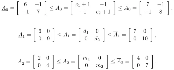
Then the interval matrix polynomial (4.6) corresponding to the open-loop system is given byF(λ) =A0+λA1+λ2A2, where
A0=
6 −1
−1 7
≤A0=
c1+ 1 −1
−1 c2+ 1
≤A0=
7 −1
−1 8
,
A1=
6 0 0 9
≤A1=
d1 0
0 d2
≤A1=
7 0
0 10
,
A2=
2 0 0 4
≤A2=
m1 0
0 m2
≤A2=
4 0 0 7
[image:17.612.103.409.574.698.2]
The system (4.2) to be solved with respect toXt0t1t2 (t0, t1, t2 ∈ {1, . . . ,4}), G
and H consists of the 64 matrix inequalities. Assuming that G = (A+A)/2 and H = 0, with the help of MATLAB, we find this system feasible. Hence, all the eigenvalues of the stable open-loop mechanical system remain in the domain (4.8) for the specified interval uncertainties. Figure 4.2 shows the roots location of the 64 matrix polynomialsFt0t1t2(λ) with respect to the Pascal’s limacon.
REFERENCES
[1] I. Gohberg, P. Lancaster, and L. Rodman. Matrix Polynomials. Academic Press, New York, 1982.
[2] A.G. Mazko. Localization of the Spectrum and Stability of Dynamic Systems. Proceedings of the Institute of Mathematics of NAS of Ukraine, Vol. 28. Institute of Mathematics of the NAS of Ukraine, Kiev, 1999 (in Russian).
[3] A.G. Mazko. Matrix Equations, Spectral Problems and Stability of Dynamic Systems. An
international book series Stability, Oscillations and Optimization of Systems (Eds. A.A. Martynyuk, P. Borne, and C. Cruz-Hernandez), Vol. 2. Cambridge Scientific Publishers Ltd, Cambridge, 2008.
[4] D. Henrion, O. Bachelier, and M. Sebek.D-stability of polynomial matrices.Internat. J. Control, 74(8):355–361, 2001.
[5] D. Henrion, D. Arzelier, and D. Peaucelle. Positive polynomial matrices and improved LMI robustness conditions. Automatica, 39(8):1479–1485, 2003.
[6] P. Lancaster. Linearization of regular matrix polynomials. Electron. J. Linear Algebra, 17: 21–27, 2008.
[7] N. Higham, D.S. Mackey, and F. Tisseur. The conditioning of linearizations of matrix polyno-mials.SIAM J. Matrix Anal. Appl., 28(4):1005–1028, 2006.
[8] E.N. Antoniou and S. Vologiannidis. A new family of companion forms of polynomial matrices. Electron. J. Linear Algebra, 11: 78–87, 2004.
[9] V.N. Kublanovskaya. On the spectral problem for polynomial pencils of matrices.Zap. Nauchn. Sem. Leningrad. Otdel. Mat. Inst. Steklov. (LOMI), 80:83–97, 1978.
[10] D. Henrion, M. Sebek, and V. Kucera. Positive polynomials and robust stabilization with fixed-order controllers. IEEE Trans. Automat. Control, 48(7):1178–1186, 2003.
[11] F.R. Gantmaher. The Theory of Matrices. Moskow, Nauka, 1988 (in Russian).
[12] B.T. Polyak and P.S. Shcherbakov. Robust Stability and Control. Moskow, Nauka, 2002 (in Russian).
[13] T.E. Djaferis.Robust Control Design: a Polynomial Approach. Kluver, Boston, 1995. [14] J. Ackermann. Robust Control. Systems with Uncertain Physical Parameters. Springer Verlag,