EXPORT DIVERSIFICATION AND ECONOMIC GROWTH IN ASEAN | Sunaryati | JESP: Jurnal Ekonomi & Studi Pembangunan 1207 3429 1 SM

(1)

Jurnal Ekonomi dan Studi Pembangunan Volume 16, Nomor 2, Oktober 2015, hlm.119-131

EXPORT DIVERSIFICATION AND ECONOMIC

GROWTH IN ASEAN

Sunaryati

Faculty of Islamic Economics and Business, Sunan Kalijaga State Islamic University Jln. Marsda Adisucipto, Yogyakarta, Daerah Istimewa Yogyakarta 55281, Indonesia

Phone: +62 274 589621. Correspondence E-mail: s_nartie@yahoo.com

Received: December 2014; accepted: September 2015

Abstract:This paper tries to assess empirically the relationship between export diversification and economic growth on selected countries in ASEAN. Using annual data or time-series over the period 1989 to 2010 and econometric techniques (Granger causality and cointegration) are applied to test the relationship between export diversification and economic growth. The result show that, in case of Indonesia and Malaysia, there are exist uni-directional causality from GDP to export diversification. For Singapore and Thailand, the results show that there are no causal relationship between export diversification and economic growth.

Keywords:export diversification, economic growth, causality, ASEAN JEL Classification:F13, F43, O40

Abstrak:Tulisan ini mencoba mengkaji secara empiris hubungan antara diversifikasi ekspor dan pertumbuhan ekonomi di negara yang dipilih di ASEAN. Dengan menggunakan data tahunan atau time series selama periode 1989 sampai 2010 dan teknik ekonometrik (Granger kausalitas dan kointegrasi) yang diterapkan untuk menguji hubungan antara diversifikasi ekspor dan pertumbuhan ekonomi. Hasil penelitian menunjukkan bahwa, dalam kasus Indonesia dan Malaysia, ada ada uni-directional kausalitas dari PDB untuk ekspor diversifi-kasi. Untuk Singapura dan Thailand, hasil menunjukkan bahwa tidak ada hubungan sebab akibat antara diversifikasi ekspor dan pertumbuhan ekonomi.

Kata kunci:diversifikasi ekspor, pertumbuhan ekonomi, kausalitas, ASEAN Klasifikasi JEL:F13, F43, O40

INTRODUCTION

The dependence on primary-product exports has been frequently mentioned as one of the main features of developing nations. As stated by Todaro and Smith (2006), less developed countries (LDCs) tend to specialize in the pro-duction of primary products, instead of second-ary and tertisecond-ary activities. Consequently, exports of primary products play a very signifi-cant role in terms of foreign exchange genera-tion in these countries, tradigenera-tionally represent-ing a significant share of their gross national product. Specially in the case of the non-mineral primary products exports, markets and prices are frequently unstable, leading to a high degree of exposure to risk and uncertainty for

the countries that rely on them (Todaro and Smith 2006). Primary-products exports have been characterized by relatively low income elasticity of demand and inelastic price elastic-ity, being fuels, certain raw materials, and manufactured goods, some exceptions that exhibit relatively high income elasticity (Todaro and Smith, 2006).

(2)

compli-cated by the fact that many of the LDCs have incurred in deficits on their balance of pay-ments, due to their import demands of capital goods, intermediate goods, and consumer pro-ducts that their industrial expansion requires. Furthermore, LDCs are usually more depend-ent on trade than developed nations, in terms of its share in national income.

Export diversification entails changing the composition of a country s export mix, being it directly related to the structure of the economy and how it changes as development proceeds . The underlying consideration behind export diversification as a possible developmental strat-egy is related to the expectation of achieving stability-oriented and growth-oriented policy objectives (Ali et al. 1991). A broader exports base, coupled with a special promotion of those commodities with positive price trends, should be beneficial for growth. Hence, the value-added export commodities would be stimulated, by means of additional processing and marketing activities. A country s degree of diversification is usually considered as dependent upon the number of commodities within its export mix, as well as on the distribution of their individual shares.

The United Nations Economic and Social Commission for Asia and the Pacific (ESCAP) has stated that for small, low-income economies such as the least developed countries (LDCs), reasonable development goals cannot be limited to primary products exports. Diversification, both in terms of non-traditional and tradi-tional commodities, is considered as an ele-ment of utmost importance for growth and de-velopment (ESCAP 2004). It has also been fre-quently stated that growth and export diversi-fication may be linked. Besides structural changes of an economy, as Al-Marhubi (2000) points out, traditional development models propose that economic growth also implies a shift from dependence on primary exports to-wards diversified manufactured exports. An-other interesting concept is linked to the so-called graduation concept addressed by empirical studies such as the ones conducted by Michaely (1977) and Moschos (1989). It suggests that the process of graduation from develop-ing to developed status should be joined by a structural change of exports toward diversity

(Amin Gutierrez de Pineres and Ferrantino, 1997a). This would suggest that the connection between exports and growth enters, when a certain level of development is attained.

Against this background, this study intends to examine the impact of export diversi-fication (DX) on economic growth in selected ASEAN Economies. Particularly, to examine the relationship betweenDXand economic growth. The relation between export diversification and economic growth has been analyzed in a wide number of empirical studies. The possible influ-ence of export diversification on growth is examined by Amin Gutierrez de Pineres and Ferrantino (1997a), by analyzing the Chilean experience within the period 1962 1991. They study the possible link between diversification, export growth and aggregate development, by constructing different measures of diversifica-tion and structural change in exports. These measures are afterward used to test different relationships among the structure of exports and export growth. Two different interesting findings are reported: first of all, a link between the domestic economic performance and diver-sification is reported, suggesting that diversifi-cation in Chile has taken place mostly during times of internal crisis or external shock. Sec-ondly, that the new products most successfully introduced in that country were mainly pri-mary products (such as tobacco, coffee and tea, and dairy products) while a number of manu-factures (like plastics, manufactured fertilizers, electrical and non-electrical machinery) have shown less dynamism. Their study also proposed that export diversification, in the long run, has boosted Chilean growth performance.

(3)

influenced by stimulating the accumulation of capital.

Agosin s study (2006) investigates whether export diversification has any explanatory power in a standard empirical model of growth. Cross-sectional data in the 1980 2003 periods is considered, for a sample of ASEAN and Latin American countries. It is suggested that export growth by itself does not appear to be relevant for growth, while export growth together with diversification appears to be relevant. This argument is supported by the fact that the interactive variable (measuring diversification and export growth) showed the expected sign and was highly significant, providing the strongest explanatory power. Export diversifi-cation is supposed to contribute to growth through two different channels, namely, the portfolio effect less export volatility- and the widening of comparative advantages, as a result of a more diversified economy.

Klinger and Lederman (2004) estimating the Herfindahl index on the log of income per capita and its squared term find a nonlinear relationship which suggests that countries diversify their export structure up to some point in their development after which get more con-centrated in their exports. To test whether the change brings higher growth rate, the squared term of the Herfindahl index is added into the regression. So in another estimation of the growth rate the squared term of the Herfindahl index will be added as an explanatory variable. The finding of a U-shaped relation of export concentration on economic growth would mean that for some countries export concentration is more beneficial than diversification.

Hesse (2008) together with the World Bank s Commission on Growth and Development using the system GMM estimator for a sample of 99 countries and Herfindahl index of export con-centration studies the impact of export concen-tration on economic growth of countries based on augmented Solow model in the period of 1961-2000. Adding the squared term of the index he finds some evidence of nonlinearity in the relationship, but the coefficients on the squared index are not significant in the work.

Theoretical Framework. Export depend-ency on primary products of a country can be reduced through diversification of the export

portfolio. However, export diversification can take place in different forms and dimensions and thus its analysis can be undertaken at dif-ferent levels. Usually, by changing the shares of commodities in the existing export mix, or by including new commodities in the export port-folio, a country can attain export diversification. In this context, there are two well-known forms of export diversification that are common in the trade literature, namely, horizontal and vertical diversification. While horizontal diversification entails alteration of the primary export mix in order to neutralize the volatility of global com-modity prices, vertical diversification involves contriving further uses for existing and new innovative commodities by means of value-added ventures such as processing and mar-keting. It is expected that vertical diversification could augment market prospects for raw mate-rials that may compliment economic growth and thus lead to further stability as processed commodities tend to have more stable prices than raw materials.

Export diversification can be categorized into two types, the horizontal diversification and vertical diversification. The former refers to diversity of product across different type of industry, while the latter covers diversity of product within the same industry i.e. value-added ventures in further downstream activi-ties. Both type of diversification is expected to positively induce economic growth (Kenji & Mengistu, 2009).

There are many way through which export diversification promotes economic growth. Export diversification could positively affect economic growth by reducing the dependency on limited number of commodities (Herzer and Nowak-Lehmann, 2006). This argument is par-ticularly true in the case of commodity-depend-ent developing countries, where overdepend-ence on agricultural sector could according to the Prebisch-Singer thesis reduce the terms of trade. The basic reason for this due to Hesse (2008) is the high degree of price volatility of commodity products.

(4)

theory, there are three main features of modern market behaviour.First, the increasing dynamic features of production factors and national poli-cies to influence the production capacity to grow with increasing return. Second, the expansions of trade model from perfect compe-tition to the imperfect compecompe-tition especially the monopolistic competition. This is partially related to the first factor, whereby increasing intensity of trade liberalization among nations and mobilization of production factors have enable firms in one country to expand their production without being constrained by diminishing return Krugman & Obstfeld (2003). This arguments in contrast to the classical trade theory implies that could involve in various production activities without confining to their comparative advantage (Arip, Yee, & Karim, 2010).

While the aforementioned two factors ex-plain the market behaviour from the supply side, the third characteristic of modern trade theory is attributed to the demand side. This is reflected by domestic market peculiarities across different countries, which are not fixed and varies in various aspects such as taste, average income, knowledge, gender, age, cul-ture and geographical division. While produc-tion in each particular country tries to meets unique characteristic of domestic market de-mand, it also enters symmetrically into the international market demand and subsequently offers the market with goods and services, which are different in the form of functionali-ties, taste, design, ingredient, quality, and appearances. This is termed as the home mar-ket´ effects on the pattern of trade by Krugman (1980). According to Krugman (1980) a country tends to export those goods for which they have relatively large domestic market.

RESEARCH METHOD

Empirical Framework

This paper use time-series techniques of cointe-gration and Granger causality tests to examine the long-run relationship and dynamic interac-tions among the variables of interest. Since these methods are now well known, we men-tion only those aspects that are relevant in our

study. Firstly, for proper model specification, we conduct the unit root and cointegration tests. We apply group unit root test, such as: Levin, Lin and Chu t (assumes common unit root process), lm, Pesaran and Shin W-Stat, Augmented Dickey-Fuller (ADF) and Phillips-Perron (PP) unit root tests (assumes individual unit root process) for determining the variables orders of integration. Then, to test for cointe-gration, we employ a vector autoregressive (VAR) based approach of Johansen (1988) and Johansen & Juselius (1990), henceforth the JJ cointegration test. Since the results of the JJ cointegration test tend to be sensitive to the order ofVAR, following Hall (1989) and Johan-sen (1992), we specify the lag length that renders the error terms serially uncorrelated.

Having implemented unit root and cointe-gration tests, we proceed to specification and estimation of Granger causality. In particular, the findings that the variables are non-station-ary and are not cointegrated suggest the use of Granger causality of VARmodel in first differ-ences. However, if they are cointegrated, a vector error correction model (VECM) or a level VAR can be used (Engle & Granger, 1987: 251-276). According to Granger representation theo-rem, for any cointegrated series, error correc-tion term must be included in the model. Engle & Granger (1987) and Toda & Phillips (1993) indicate that omitting this error correction term (ECT) in the model, leads to model misspecifi-cation. Through theECT, theECMopens up an additional channel for Granger-causality to emerge that is completely ignored by the stand-ard Granger and Sims tests (Masih, A. M. M. & Masih, R; 1999).

(5)

0 1 1 2 3 k i i t k

GDP

DX

EMP

CAP



 





  









  









  



 











  











  









  







0 1 2 3 1 t

GDP

v

DX

v

EMP

v

CAP

_

v





 





 





 









 





 





 

(1)

where GDP is gross domestic product, DX is export diversification index, EMP is employ-ment, andCAPis capital expenditure.

Data Description

The data used in this study are annual data for the period of 1989 to 2010.The data set is com-piled into a panel data from sources as the International Financial Statistics of theIMF, the World Integrated Trade Solution of the World Bank and the Key Indicators of the ASEAN Development Bank (ADB). In this paper, the focal variables are gross domestic product (GDP) and the export diversification index (DX). However focusing on these two variables in a bivariate context may not be satisfactory since they may be driven by common factors thus the results will be misleading. Following Herzer and Nowak-Lehmann (2006), we also include capital expenditure (CAP) and the number of people employed (EMP) as control variables.

Export diversification is held to be im-portant for developing countries because many developing countries are often highly depend-ent on relatively few primary commodities for their export earning. Unstable prices of their commodities may subject a developing country exporter to serious terms of trade shocks. Since the covariation in individual commodity prices is less than perfect, diversification into new primary export product is generally view as appositive development. The strongest positive effect are normally associated with diversifica-tion into manufactured goods, and its benefit include higher and more stable export earnings,

job creation, and learning effects and the devel-opment of new skills and infrastructure that would facilitate the development of even newer export product. The export diversification index (DX) for a country is defined as:



ij i



/

2

j

sum

h

x

DX





(2)

Wherehijis the share of commodityiin the total exports of country j and xi is the share of the commodity in world exports. The related meas-ure used by UNCTAD is the concentration index or Hirschman (H) index, which is calcu-lated using the shares of all three-digit products in a country s exports:























2 t

j

sqrt

sum

X

x

H

(3)

Where xiis country js export in product i (at three digit classification) and Xt is country js total export. The index has been normalized to account for the number of three digit product that could be exported. Thus, maximum value of the index is 239 (the number of individual three digit products in SITC revision 2), and its minimum (theoretical value) is zero, for country with no export. The lower the index, the less concentrated are country s export.

RESULTS AND DISCUSSION

Unit Root Tests

(6)

Cointegration Tests

In order to capture dynamic relationship among the observed variables, their cointegration rela-tionship was tested trough multivariate meth-odology proposed by Johansen (1990) and Johansen and Juselius (1991). Johansen (1991) modeled time series as a reduced rank regres-sions in which they computed the maximum likelihood estimates in the multivariate cointe-gration model with Gaussians errors. The ad-vantage of this technique is that it allows one to draw a conclusion about the number of cointe-grating relationship among observed variables. Since all the data series in the model were inte-grated processes of order one orI(1), the linear combination (cointegrating vectors) of one or more of these series may exhibit long run rela-tionship. The maximum eigenvalue test and trace test was employed to established the number of cointegrating vectors. The results are presented in table 5 8 (see Appendix). The optimal lag length (p) is determined using Schwartz Information Criterion (SIC), which indicates an optimal lag length of one year.

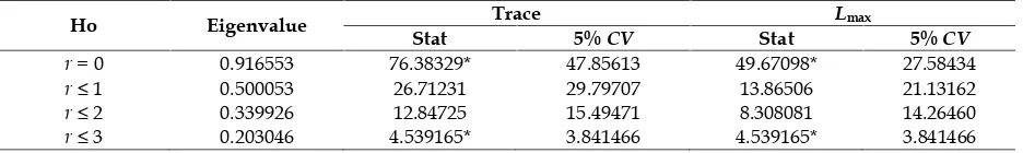
In the case of Indonesia, Malaysia and Thailand, the result of trace test and maximum eigenvalue test both indicate that, there is one cointegrating vector at 5% level of significance. For Singapore, the result of trace test and maximum eigenvalue test both indicate that, there is two cointegrating vector at 5% level of significance.

Granger Causality Tests

As discussed above that there is co-integration between the variables, so the next step is to test for the direction of causality using the vector error correction model. Firstly, we present the traditional Granger causality results for each country as in table 9 12 (see Appendix). In case of Indonesia, the result in table 9 show that GDP does Granger causeDX at7% level of sig-nificance. So, there is exist unidirectional cau-sality from GDP to Export Diversification. For Malaysia, the estimation result indicated that we reject the null hypothesis of GDP does not Granger cause DX and conclude that there is exists uni-directional causality between Eco-nomic Growth and Export Diversification at the 1% level of significance.

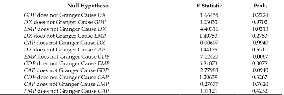
Table 11 & 12 show estimation result for Singapore and Thailand. The result indicate that we cannot reject both of the Ho of GDP does not Granger causeDX and the Ho of DX does not Granger cause GDP at 5% level of significance. Therefore, we accept the Ho, and conclude that GDP does not Granger cause export diversification and export diversification does not Granger causeGDP. In other word, we can say that both variables are independent.

Vector Error Correction Model

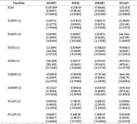
In order to check the stability of the model we have estimated the vector error correction (VEC) model. The results ofVECmodel are pre-sented in Table 13 16 (see Appendix). For Indonesia, the results indicate that the error cor-rection term forGDPbears the correct sign i.e. it is negative and statistically significant at 5 per-cent significant level, implying that there exist a long run causality running from export diversification to GDP.

Meanwhile, in case of Malaysia, coefficient of error term with export diversification as dependent variable is statistically significant, yet the sign is positive (not correct). This find-ing is in accordance with result of cointegration test implying that only one cointegration equa-tion running in the long run.

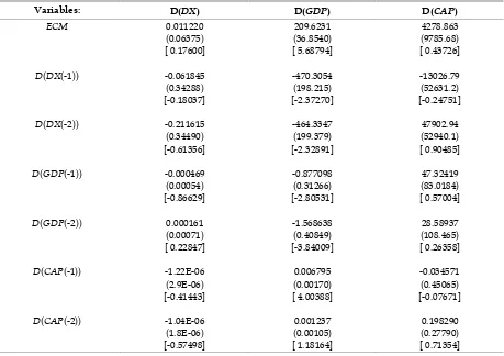
For Singapore (table 15), we know that coefficient of error term withGDPas dependent variable is statistically significant, but the sign is positive (not correct).

Otherwise, coefficient of error term with export diversification as dependent variable is not significant. These results suggest that no long run relationship between export diversifi-cation and economic growth.

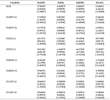
In case of Thailand, both of the coefficient of error term with GDP (DX) as dependent variable are not statistically significant, implying that no long run relationship between export diversification and economic growth, vice versa (table 16).

CONCLUSION

(7)

Econo-mies (Indonesia, Malaysia, Singapore and Thailand) using annual data over the period 1989 to 2010. The unit root properties of the data were examined using group unit root test, such as: Levin, Lin and Chu t (assumes com-mon unit root process), lm, Pesaran and Shin W-Stat, Augmented Dickey-Fuller (ADF) and Phillips-Perron (PP) unit root tests (assumes individual unit root process) after which the cointegration and causality tests were con-ducted. The error correction models were also estimated in order to examine the short run dynamics. The major findings include the fol-lowing:

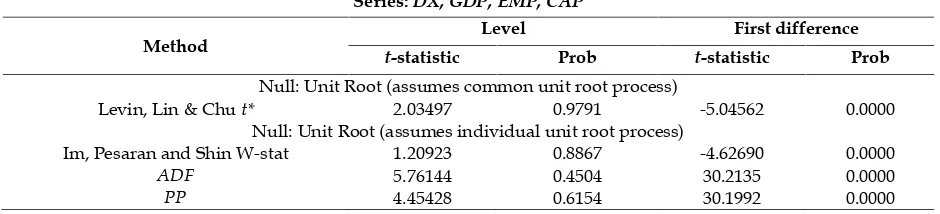
The unit root tests clarified that all varia-bles (DX, GDP, EMP and CAP) are non station-ary at the level data but found stationstation-ary at the first difference. Therefore, for all countries, the series were found to be integrated of order one. Furthermore, cointegration tests indicate that there exists a long run equilibrium relationship between exports diversification and GDP in all countries as confirmed by Johansen cointegra-tion test results.

The Granger causality test finally con-firmed that in case of Indonesia and Malaysia, there are exist uni-directional causality from GDP to export diversification. For Singapore and Thailand, the results show that there are no causal relationship between export diversifica-tion and economic growth.

REFERENCES

Agosin, M. P. (2007). Export diversification and growth in emerging economies, Working Paper No.233. Universidad de Chile: De-partmento de Economia.

Al Marhubi, F. A. (2000). Export diversification and growth: an empirical investigation. Applied Economics Letters, 7,559-562. Amin Gutiérrez de Piñeres, Sheila, and Michael

J. Ferrantino. (1997a). Export diversifica-tion and structural change: some com-parisons for Latin America. The Interna-tional Executive, Vol. 39 No. 4, July/Au-gust, 465-477.

Arip, Mohammad Aendy, Yee, Lau Sim and Abdul Karim, Bakri. (2010). Export

diversification and economic growth in Malaysia,MPRAWorking PaperNo. 20588. ASEAN Development Bank. Key indicator for

Asia and Pacific, (2011).

Engle, R. F., & Granger, C. W. J. (1987). Cointe-gration and error correction: representa-tion, estimarepresenta-tion, and testing.Econometrica, 55, 251-276

Hall, S. G. (1989). Maximum likelihood estima-tion of cointegrating vectors: An Example of Johansen s Procedure.Oxford Bulletin of Economics and Statistics, 51, 213-218. Hesse, H. (2008). Export diversification and

eco-nomic growth, Working Paper No. 21. the Commission on Growth and Develop-ment.

Herzer, D., & Lehmann, N. (2006). What does export diversification do for a growth? An Econometric Analysis. Applied Economic Letters, 38(15), 1825-1838.

International Monetary Fund. (2012). World Economic Outlook Database.

Johansen, S. and Juselius, K. (1990). Maximum likelihood estimation and inference on cointegration with applications to the demand for money. Oxford Bulletin of Economics and Statistics.

Kenji, Y., & Mengistu, A. A. (2009). The impacts of vertical and horizontal export diversi-fication on growth: an empirical study on factors explaining the gap between Sub-Sahara Africa and East Asia's Per-formances.Ritsumeikan International Affair, 17, 41.

Klinger, Bailey and Daniel Lederman. (2004): Discovery and development: an empirical exploration of new products. Policy Research Working Paper No. 3450, World Bank, November.

Krugman, P. (1980). Scale economies, product differentiation, and the pattern of trade. The American Economic Review, 70(5), 950. Krugman, P., & Obstfeld, D. 2003).International

economics: theory and policy(754, Trans. 6th ed.). Boston: Pearson Education, Inc. Masih, A. M. M., & Masih, R. (1999). Are

(8)

Evidence Based on ASEAN Emerging Stock Markets, Pacific-Basin Finance Journal, 7, 251-282.

Michaely, M. (1977). Exports and growth: an empirical investigation. Journal of Devel-opment Economics4: 49-53.

Moschos, D. (1989). Export expansion, growth and the level of economic development:

an empirical analysis. Journal of Develop-ment Economics,30: 93-102.

Toda, H. Y., & Phillips, P. C. B. (1993). Vector autoregression and causality. Economet-rica, 59, 229-255.

World Bank. (2011). The World integrated trade solution: Trade Indicator.

[image:8.595.51.520.278.385.2]

APPENDIX

Table 1. Group unit root test results: Indonesia

Series:DX, GDP, EMP, CAP

Method

Level First difference

t-statistic Prob t-statistic Prob

Null: Unit Root (assumes common unit root process)

Levin, Lin & Chu t* 1.38054 0.9163 -8.51243 0.0000

Null: Unit Root (assumes individual unit root process)

Im, Pesaran and Shin W-stat 2.81844 0.9976 -7.40062 0.0000

ADF 7.73178 0.4601 56.7549 0.0000

PP 8.41325 0.3942 56.7549 0.0000

Table 2. Group unit root test results: Malaysia

Series:DX, GDP, EMP, CAP

Method

Level First difference

Levin, Lin & Chu t* -1.11401 0.1326 -4.82959 0.0000

ADF 7.75127 0.4581 37.6187 0.0000

PP 10.5651 0.2276 123.700 0.0000

Table 3. Group unit root test results: Singapore

Series:DX, GDP, EMP, CAP

Method Level First difference

Levin, Lin & Chut* 2.03497 0.9791 -5.04562 0.0000

ADF 5.76144 0.4504 30.2135 0.0000

[image:8.595.49.519.581.688.2]

(9)

[image:9.595.76.546.87.193.2]

Table 4. Group unit root test results: Thailand

Series:DX, GDP, EMP, CAP

Method Level First difference

t-statistic Prob t-statistic Prob

Levin, Lin & Chut* -1.34370 0.0895 -6.46399 0.0000

ADF 18.3928 0.0185 44.0740 0.0000

[image:9.595.75.546.232.304.2]

PP 39.0924 0.0000 41.2199 0.0000

Table 5. Johansen cointegration tests: Indonesia

Ho Eigenvalue Trace Lmax

Stat 5%CV Stat 5%CV

r= 0 0.682765 45.54770 47.85613 22.96226 27.58434

r 1 0.467131 22.58544 29.79707 12.58959 21.13162

r 2 0.242084 9.995853 15.49471 5.543660 14.26460

r 3 0.199573 4.452193* 3.841466 4.452193* 3.841466

[image:9.595.80.549.356.427.2]

* denote rejection of the hypothesis at the 0.05 level

Table 6. Johansen cointegration tests: Malaysia

Ho Eigenvalue Trace Lmax

Stat 5%CV Stat 5%CV

r= 0 0.818141 56.39197* 47.85613 34.09049* 27.58434

r 1 0.492489 22.30147 29.79707 13.56476 21.13162

r 2 0.326337 8.736718 15.49471 7.900492 14.26460

r 3 0.040949 0.836226 3.841466 0.836226 3.841466

Table 7. Johansen Cointegration tests: Singapore

Ho Eigenvalue Trace Lmax

r= 0 0.942077 93.11025* 47.85613 56.97270* 27.58434

r 1 0.766412 36.13754* 29.79707 29.08390* 21.13162

r 2 0.210727 7.053644 15.49471 4.732864 14.26460

r 3 0.109560 2.320780 3.841466 2.320780 3.841466

Table 8. Johansen Cointegration tests: Thailand

Ho Eigenvalue Trace Lmax

r= 0 0.916553 76.38329* 47.85613 49.67098* 27.58434

r 1 0.500053 26.71231 29.79707 13.86506 21.13162

r 2 0.339926 12.84725 15.49471 8.308081 14.26460

r 3 0.203046 4.539165* 3.841466 4.539165* 3.841466

[image:9.595.80.553.480.551.2] [image:9.595.80.548.604.674.2]

(10)

[image:10.595.53.519.87.237.2]

Table 9. Granger causality for Indonesia

Null Hypothesis F-Statistic Prob.

GDPdoes not Granger CauseDX 3.01597 0.0793

DXdoes not Granger CauseGDP 1.06480 0.3695

EMPdoes not Granger CauseDX 1.64810 0.2254

DXdoes not Granger CauseEMP 1.22905 0.3204

CAPdoes not Granger CauseDX 0.13425 0.8754

DXdoes not Granger CauseCAP 6.65131 0.0086

EMPdoes not Granger CauseGDP 0.34151 0.7161

GDPdoes not Granger CauseEMP 3.85788 0.0445

CAPdoes not Granger CauseGDP 0.29567 0.7483

GDPdoes not Granger CauseCAP 1.03967 0.3777

CAPdoes not Granger CauseEMP 2.14397 0.1517

[image:10.595.57.516.270.422.2]

EMPdoes not Granger CauseCAP 0.99266 0.3937

Table 10. Granger causality for Malaysia

Null Hypothesis F-Statistic Prob.

EMP does not Granger CauseDX 1.53117 0.2482

Table 11. Granger causality for Singapore

Null Hypothesis F-Statistic Prob.

Table 12. Granger causality for Thailand

Null Hypothesis F-Statistic Prob.

[image:10.595.56.517.458.613.2] [image:10.595.58.517.654.756.2]

(11)

[image:11.595.86.546.170.584.2]

Table 13. Multivariate Granger causality tests based onVECM: Indonesia

Variables D(GDP) D(DX) D(EMP) D(CAP)

ECM -0.837089* -3.21E-05 -0.004431 -125.2820

[image:11.595.77.546.633.766.2]

(0.08507) (9.9E-05) (0.01048) (145.899)

[-9.84034] [-0.32401] [-0.42286] [-0.85869]

D(GDP(-1)) 0.433721 -8.87E-05 0.009173 61.08693

(0.12778) (0.00015) (0.01574) (219.148)

[ 3.39440] [-0.59584] [ 0.58280] [ 0.27875]

D(GDP(-2)) 0.433905 0.000387 0.015576 346.1866

(0.10803) (0.00013) (0.01331) (185.290)

[ 4.01636] [ 3.07488] [ 1.17038] [ 1.86835]

D(DX(-1)) 212.8895 0.029009 -8.544325 -929034.5

(244.096) (0.28453) (30.0690) (418649.)

[ 0.87215] [ 0.10196] [-0.28416] [-2.21912]

D(DX(-2)) -208.3858 0.286727 6.301253 -533728.0

(288.695) (0.33651) (35.5629) (495141.)

[-0.72182] [ 0.85206] [ 0.17719] [-1.07793]

D(EMP(-1)) -35.88820 -0.003854 -0.761148 -4442.481

(4.13899) (0.00482) (0.50986) (7098.79)

[-8.67076] [-0.79888] [-1.49285] [-0.62581]

D(EMP(-2)) -32.21117 -0.005264 -0.004763 -2191.842

(3.25034) (0.00379) (0.40039) (5574.66)

[-9.91010] [-1.38950] [-0.01189] [-0.39318]

D(CAP(-1)) 0.000745 1.70E-07 2.65E-05 0.019336

(0.00018) (2.1E-07) (2.2E-05) (0.30883)

[ 4.13524] [ 0.81010] [ 1.19610] [ 0.06261]

D(CAP(-2)) 0.000672 3.46E-08 1.00E-05 -0.021338

(0.00017) (1.9E-07) (2.0E-05) (0.28533)

[ 4.04006] [ 0.17852] [ 0.48984] [-0.07478]

Notes: standard errors in () &t-statistic in []

Table 14. Multivariate Granger Causality Tests Based on VECM: Malaysia

Variables D(GDP) D(DX) D(EMP) D(CAP)

ECM -0.106100 0.000351* 0.001219 10.02449

(0.12197) (8.5E-05) (0.00329) (37.0443)

[-0.86990] [ 4.15761] [ 0.37007] [ 0.27061]

D(GDP(-1)) 0.947231 -0.001924 -0.003210 -69.70183

(0.55322) (0.00038) (0.01494) (168.023)

(12)

D(GDP(-2)) 0.546984 -0.001139 -0.006571 -4.607880

[image:12.595.57.516.427.751.2]

(0.85742) (0.00059) (0.02316) (260.416)

[ 0.63794] [-1.91661] [-0.28370] [-0.01769]

D(DX(-1)) 904.7039 -0.879051 -6.106484 -60882.36

(351.174) (0.24330) (9.48572) (106659.)

[ 2.57623] [-3.61298] [-0.64376] [-0.57082]

D(DX(-2)) -77.15913 0.067723 -5.020546 40322.15

(414.663) (0.28729) (11.2007) (125941.)

[-0.18608] [ 0.23573] [-0.44824] [ 0.32017]

D(EMP(-1)) -29.40748 0.038615 -0.173311 2209.854

(20.1452) (0.01396) (0.54415) (6118.50)

[-1.45978] [ 2.76669] [-0.31850] [ 0.36118]

D(EMP(-2)) -3.384447 0.006708 -0.385816 -3700.354

(13.5038) (0.00936) (0.36476) (4101.37)

[-0.25063] [ 0.71697] [-1.05774] [-0.90222]

D(CAP(-1)) 0.000113 -1.12E-06 3.03E-05 0.124685

(0.00134) (9.3E-07) (3.6E-05) (0.40655)

[ 0.08421] [-1.21305] [ 0.83731] [ 0.30669]

D(CAP(-2)) 0.000588 -1.01E-06 4.36E-06 -0.128248

(0.00114) (7.9E-07) (3.1E-05) (0.34720)

[ 0.51462] [-1.27642] [ 0.14133] [-0.36938]

Notes: standard errors in () &t-statistic in []

Table 15. Multivariate Granger Causality Tests based onVECM: Singapore

Variables: D(DX) D(GDP) D(CAP)

ECM 0.011220 209.6231 4278.863

(0.06375) (36.8540) (9785.68)

[ 0.17600] [ 5.68794] [ 0.43726]

D(DX(-1)) -0.061845 -470.3054 -13026.79

(0.34288) (198.215) (52631.2)

[-0.18037] [-2.37270] [-0.24751]

D(DX(-2)) -0.211615 -464.3347 47902.94

(0.34490) (199.379) (52940.1)

[-0.61356] [-2.32891] [ 0.90485]

D(GDP(-1)) -0.000469 -0.877098 47.32419

(0.00054) (0.31266) (83.0184)

[-0.86629] [-2.80531] [ 0.57004]

D(GDP(-2)) 0.000161 -1.568638 28.58937

(0.00071) (0.40849) (108.465)

[ 0.22847] [-3.84009] [ 0.26358]

D(CAP(-1)) -1.22E-06 0.006795 -0.034571

(2.9E-06) (0.00170) (0.45065)

[-0.41443] [ 4.00388] [-0.07671]

D(CAP(-2)) -1.04E-06 0.001237 0.198290

(1.8E-06) (0.00105) (0.27790)

[-0.57498] [ 1.18164] [ 0.71354]

(13)

[image:13.595.86.546.87.503.2]

Table 16. Multivariate Granger causality tests based on VECM: Thailand

Variables: D(GDP) D(DX) D(EMP) D(CAP)

ECM 0.785929 -0.000879 0.043637 0.344911

(0.82828) (0.00050) (0.00938) (1.46114)

[ 0.94887] [-1.76146] [ 4.65124] [ 0.23606]

D(GDP(-1)) -0.765429 0.001383 -0.061697 0.044245

(1.56139) (0.00094) (0.01769) (2.75439)

[-0.49022] [ 1.47003] [-3.48849] [ 0.01606]

D(GDP(-2)) -0.673741 0.000162 -0.001264 0.694222

(0.63732) (0.00038) (0.00722) (1.12427)

[-1.05715] [ 0.42128] [-0.17510] [ 0.61749]

D(DX(-1)) 642.7876 0.123443 29.38906 587.9058

(584.861) (0.35236) (6.62467) (1031.73)

[ 1.09904] [ 0.35033] [ 4.43630] [ 0.56982]

D(DX(-2)) 1312.402 -1.664573 66.07803 0.120507

(1656.58) (0.99804) (18.7640) (2922.32)

[ 0.79224] [-1.66785] [ 3.52154] [ 4.1e-05]

D(EMP(-1)) 10.36249 -6.73E-05 -0.298477 -2.761696

(12.3958) (0.00747) (0.14041) (21.8671)

[ 0.83597] [-0.00902] [-2.12580] [-0.12629]

D(EMP(-2)) 0.943376 0.012452 -0.456162 -3.930901

(15.6535) (0.00943) (0.17731) (27.6139)

[ 0.06027] [ 1.32039] [-2.57273] [-0.14235]

D(CAP(-1)) 0.544919 -0.000380 0.018851 0.480540

(0.45761) (0.00028) (0.00518) (0.80725)

[ 1.19081] [-1.37804] [ 3.63688] [ 0.59528]

D(CAP(-2)) 0.563680 -0.000676 0.019374 0.043864

(0.59870) (0.00036) (0.00678) (1.05614)

[ 0.94151] [-1.87351] [ 2.85689] [ 0.04153]