Elementary Linear Algebra - Area

(1)

Chapter 1

LINEAR EQUATIONS

1.1 Introduction to linear equations

Alinear equation innunknownsx1, x2,· · ·, xn is an equation of the form

a1x1+a2x2+· · ·+anxn=b,

wherea1, a2, . . . , an, b are given real numbers.

For example, with x and y instead of x1 and x2, the linear equation 2x+ 3y = 6 describes the line passing through the points (3,0) and (0,2). Similarly, with x, y and z instead of x1, x2 and x3, the linear equa-tion 2x + 3y + 4z = 12 describes the plane passing through the points (6,0,0),(0,4,0),(0,0,3).

Asystemofmlinear equations in nunknownsx1, x2,· · ·, xnis a family

of linear equations

a11x1+a12x2+· · ·+a1nxn = b1

a21x1+a22x2+· · ·+a2nxn = b2

.. .

am1x1+am2x2+· · ·+amnxn = bm.

We wish to determine if such a system has a solution, that is to find out if there exist numbersx1, x2,· · ·, xn which satisfy each of the equations

simultaneously. We say that the system is consistent if it has a solution. Otherwise the system is calledinconsistent.

(2)

Note that the above system can be written concisely as

n

X

j=1

aijxj =bi, i= 1,2,· · ·, m.

The matrix



   

a11 a12 · · · a1n

a21 a22 · · · a2n

..

. ...

am1 am2 · · · amn



   

is called thecoefficient matrix of the system, while the matrix



   

a11 a12 · · · a1n b1

a21 a22 · · · a2n b2

..

. ... ...

am1 am2 · · · amn bm



   

is called theaugmented matrixof the system.

Geometrically, solving a system of linear equations in two (or three) unknowns is equivalent to determining whether or not a family of lines (or planes) has a common point of intersection.

EXAMPLE 1.1.1 Solve the equation

2x+ 3y= 6.

Solution. The equation 2x + 3y = 6 is equivalent to 2x = 6−3y or

x= 3−3

2y, wherey is arbitrary. So there are infinitely many solutions.

EXAMPLE 1.1.2 Solve the system

x+y+z = 1

x−y+z = 0.

Solution. We subtract the second equation from the first, to get 2y = 1 and y = 1

2. Then x =y−z= 1

2 −z, where z is arbitrary. Again there are

infinitely many solutions.

EXAMPLE 1.1.3 Find a polynomial of the formy=a0+a1x+a2x2

+a3x3

(3)

1.1. INTRODUCTION TO LINEAR EQUATIONS 3

Solution. Whenx has the values−3,−1,1,2, theny takes corresponding values−2,2,5,1 and we get four equations in the unknownsa0, a1, a2, a3:

a0−3a1+ 9a2−27a3 = −2

a0−a1+a2−a3 = 2

a0+a1+a2+a3 = 5

a0+ 2a1+ 4a2+ 8a3 = 1.

This system has the unique solution a0 = 93/20, a1 = 221/120, a2 =

−23/20,

a3 =−41/120. So the required polynomial is

y = 93 20+

221 120x−

23 20x

2 − 41

120x

3 .

In [26, pages 33–35] there are examples of systems of linear equations which arise from simple electrical networks using Kirchhoff’s laws for elec-trical circuits.

Solving a system consisting of a single linear equation is easy. However if we are dealing with two or more equations, it is desirable to have a systematic method of determining if the system is consistent and to find all solutions.

Instead of restricting ourselves to linear equations with rational or real coefficients, our theory goes over to the more general case where the coef-ficients belong to an arbitrary field. A field F is a set F which possesses operations of additionand multiplication which satisfy the familiar rules of rational arithmetic. There are ten basic properties that a field must have:

THE FIELD AXIOMS.

1. (a+b) +c=a+ (b+c) for all a, b, cinF;

2. (ab)c=a(bc) for all a, b, cinF;

3. a+b=b+afor all a, binF;

4. ab=bafor all a, binF;

5. there exists an element 0 in F such that 0 +a=afor all ainF;

(4)

7. to everyainF, there corresponds anadditive inverse −ainF, satis-fying

a+ (−a) = 0;

8. to every non–zero a in F, there corresponds a multiplicative inverse a−1 inF, satisfying

aa−1 _{= 1;}

9. a(b+c) =ab+acfor all a, b, cinF;

10. 06= 1.

With standard definitions such as a−b = a+ (−b) and a

b = ab

−1 for

b6= 0, we have the following familiar rules:

−(a+b) = (−a) + (−b), (ab)−1=a−1b−1;

−(−a) = a, (a−1)−1=a;

−(a−b) = b−a, (a

b)

−1 ₌ b

a; a

b + c d =

ad+bc bd ; a

b c d =

ac bd; ab

ac = b c,

a

b c

= ac

b ; −(ab) = (−a)b=a(−b);

−a b

= −a

b = a −b;

0a = 0; (−a)−1 ₌ ₋₍_a−1₎_.

Fields which have only finitely many elements are of great interest in many parts of mathematics and its applications, for example to coding the-ory. It is easy to construct fields containing exactly p elements, where p is a prime number. First we must explain the idea of modular addition and

modular multiplication. If a is an integer, we define a (mod p) to be the

least remainder on dividingaby p: That is, ifa=bp+r, whereband r are integers and 0≤r < p, thena(mod p) =r.

(5)

1.1. INTRODUCTION TO LINEAR EQUATIONS 5

Then addition and multiplication modp are defined by

a⊕b = (a+b) (modp)

a⊗b = (ab) (modp).

For example, with p = 7, we have 3⊕4 = 7 (mod 7) = 0 and 3⊗5 = 15 (mod 7) = 1. Here are the complete addition and multiplication tables mod 7:

⊕ 0 1 2 3 4 5 6

0 0 1 2 3 4 5 6

1 1 2 3 4 5 6 0

2 2 3 4 5 6 0 1

3 3 4 5 6 0 1 2

4 4 5 6 0 1 2 3

5 5 6 0 1 2 3 4

6 6 0 1 2 3 4 5

⊗ 0 1 2 3 4 5 6

0 0 0 0 0 0 0 0

1 0 1 2 3 4 5 6

2 0 2 4 6 1 3 5

3 0 3 6 2 5 1 4

4 0 4 1 5 2 6 3

5 0 5 3 1 6 4 2

6 0 6 5 4 3 2 1

If we now letZ_p ={0,1, . . . , p−1}, then it can be proved thatZ_p forms a field under the operations of modular addition and multiplication modp. For example, the additive inverse of 3 in Z7 is 4, so we write −3 = 4 when

calculating inZ7. Also the multiplicative inverse of 3 inZ7 is 5 , so we write

3−1= 5 when calculating in _Z

7.

In practice, we writea⊕banda⊗basa+bandabora×bwhen dealing with linear equations overZ_p.

The simplest field isZ2, which consists of two elements 0,1 with addition

satisfying 1 + 1 = 0. So inZ2,−1 = 1 and the arithmetic involved in solving

equations overZ2 is very simple.

EXAMPLE 1.1.4 Solve the following system overZ2: x+y+z = 0

x+z = 1.

Solution. We add the first equation to the second to gety = 1. Thenx= 1−z= 1 +z, withzarbitrary. Hence the solutions are (x, y, z) = (1,1,0) and (0,1,1).

(6)

1.2 Solving linear equations

We show how to solve any system of linear equations over an arbitrary field, using theGAUSS–JORDANalgorithm. We first need to define some terms.

DEFINITION 1.2.1 (Row–echelon form) A matrix is in row–echelon formif

(i) all zero rows (if any) are at the bottom of the matrix and

(ii) if two successive rows are non–zero, the second row starts with more zeros than the first (moving from left to right).

For example, the matrix



  

0 1 0 0 0 0 1 0 0 0 0 0 0 0 0 0



  

is in row–echelon form, whereas the matrix



  

0 1 0 0 0 1 0 0 0 0 0 0 0 0 0 0



  

is not in row–echelon form.

The zeromatrix of any size is always in row–echelon form.

DEFINITION 1.2.2 (Reduced row–echelon form) A matrix is in re-duced row–echelon formif

1. it is in row–echelon form,

2. the leading (leftmost non–zero) entry in each non–zero row is 1,

3. all other elements of the column in which the leading entry 1 occurs are zeros.

For example the matrices

1 0 0 1

and



  

0 1 2 0 0 2 0 0 0 1 0 3 0 0 0 0 1 4 0 0 0 0 0 0



(7)

1.2. SOLVING LINEAR EQUATIONS 7

are in reduced row–echelon form, whereas the matrices



are not in reduced row–echelon form, but are in row–echelon form.

The zeromatrix of any size is always in reduced row–echelon form.

Notation. If a matrix is in reduced row–echelon form, it is useful to denote the column numbers in which the leading entries 1 occur, by c1, c2, . . . , cr,

with the remaining column numbers being denoted by cr+1, . . . , cn, where

r is the number of non–zero rows. For example, in the 4×6 matrix above, we have r= 3, c1 = 2, c2= 4, c3= 5, c4 = 1, c5 = 3, c6 = 6.

The following operations are the ones used on systems of linear equations and do not change the solutions.

DEFINITION 1.2.3 (Elementary row operations) There are three types of elementary row operationsthat can be performed on matrices:

1. Interchanging two rows:

Ri ↔Rj interchanges rows iand j.

2. Multiplying a row by a non–zero scalar:

Ri →tRi multiplies row iby the non–zero scalar t.

3. Adding a multiple of one row to another row:

Rj →Rj+tRi addst times rowito rowj.

DEFINITION 1.2.4 [Row equivalence]Matrix Aisrow–equivalentto ma-trixB ifB is obtained fromAby a sequence of elementary row operations.

EXAMPLE 1.2.1 Working from left to right,

(8)

Thus A is row–equivalent to B. Clearly B is also row–equivalent toA, by performing the inverse row–operationsR1→ 1

2R1, R2 ↔R3, R2→R2−2R3

onB.

It is not difficult to prove that ifAandBare row–equivalent augmented matrices of two systems of linear equations, then the two systems have the same solution sets – a solution of the one system is a solution of the other. For example the systems whose augmented matrices are A and B in the above example are respectively

 



x+ 2y = 0 2x+y = 1

x−y = 2

and

 



2x+ 4y = 0

x−y = 2 4x−y = 5

and these systems have precisely the same solutions.

1.3 The Gauss–Jordan algorithm

We now describe the GAUSS–JORDAN ALGORITHM. This is a process which starts with a given matrixAand produces a matrixBin reduced row– echelon form, which is row–equivalent toA. If A is the augmented matrix of a system of linear equations, thenB will be a much simpler matrix than

Afrom which the consistency or inconsistency of the corresponding system is immediately apparent and in fact the complete solution of the system can be read off.

STEP 1.

Find the first non–zero column moving from left to right, (column c1) and select a non–zero entry from this column. By interchanging rows, if necessary, ensure that the first entry in this column is non–zero. Multiply row 1 by the multiplicative inverse ofa1c1 thereby convertinga1c1 to 1. For each non–zero element aic1, i > 1, (if any) in column c1, add −aic1 times row 1 to rowi, thereby ensuring that all elements in column c1, apart from the first, are zero.

(9)

1.4. SYSTEMATIC SOLUTION OF LINEAR SYSTEMS. 9

The process is repeated and will eventually stop after r steps, either because we run out of rows, or because we run out of non–zero columns. In general, the final matrix will be in reduced row–echelon form and will have

r non–zero rows, with leading entries 1 in columnsc1, . . . , cr, respectively.

EXAMPLE 1.3.1

The last matrix is in reduced row–echelon form.

REMARK 1.3.1 It is possible to show that a given matrix over an ar-bitrary field is row–equivalent to precisely one matrix which is in reduced row–echelon form.

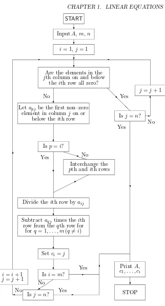
A flow–chart for the Gauss–Jordan algorithm, based on [1, page 83] is pre-sented in figure 1.1 below.

1.4 Systematic solution of linear systems.

Suppose a system ofm linear equations innunknownsx1,· · ·, xn has

aug-mented matrix A and that A is row–equivalent to a matrix B which is in reduced row–echelon form, via the Gauss–Jordan algorithm. ThenAand B

arem×(n+ 1). Suppose thatB hasr non–zero rows and that the leading entry 1 in row ioccurs in column numberci, for 1≤i≤r. Then

(10)

START

Are the elements in the

jth column on and below the ith row all zero?

Let apj be the first non–zero

element in column j on or below theith row

Subtractaqj times the ith

row from the qth row for

(11)

Also assume that the remaining column numbers arecr+1,· · ·, cn+1, where

1≤cr+1< cr+2< · · · < cn≤n+ 1.

Case 1: cr = n+ 1. The system is inconsistent. For the last non–zero

row ofB is [0,0,· · ·,1] and the corresponding equation is 0x1+ 0x2+· · ·+ 0xn= 1,

which has no solutions. Consequently the original system has no solutions.

Case 2: cr ≤n. The system of equations corresponding to the non–zero

rows ofB is consistent. First notice thatr ≤nhere. If r=n, thenc1 = 1, c2= 2,· · ·, cn=nand

B =



          

1 0 · · · 0 d1

0 1 · · · 0 d2

..

. ...

0 0 · · · 1 dn

0 0 · · · 0 0 ..

. ...

0 0 · · · 0 0



           .

There is a unique solutionx1=d1, x2 =d2,· · ·, xn=dn.

If r < n, there will be more than one solution (infinitely many if the field is infinite). For all solutions are obtained by taking the unknowns

xc1,· · ·, xcr asdependentunknowns and using the r equations

correspond-ing to the non–zero rows of B to express these unknowns in terms of the remaining independent unknowns xcr+1, . . . , xcn, which can take on

arbi-trary values:

xc1 = b1n+1−b1cr+1xcr+1− · · · −b1cnxcn

.. .

xcr = br n+1−brcr+1xcr+1− · · · −brcnxcn.

In particular, taking xcr+1 = 0, . . . , xcn

−1 = 0 and xcn = 0,1 respectively,

produces at least two solutions.

x+y = 0

(12)

Solution. The augmented matrix of the system is

A=





1 1 0

1 −1 1

4 2 1





which is row equivalent to

B =





1 0 1

2

0 1 −1 2

0 0 0



.

We read off the unique solutionx= 1

2, y=− 1 2.

(Here n = 2, r = 2, c1 = 1, c2 = 2. Also cr = c2 = 2 < 3 = n+ 1 and

r=n.)

2x1+ 2x2−2x3 = 5 7x1+ 7x2+x3 = 10 5x1+ 5x2−x3 = 5.

Solution. The augmented matrix is

A=





2 2 −2 5

7 7 1 10

5 5 −1 5





B =





1 1 0 0 0 0 1 0 0 0 0 1



.

We read off inconsistency for the original system.

(Heren= 3, r= 3, c1= 1, c2= 3. Also cr=c3 = 4 =n+ 1.)

x1−x2+x3 = 1

(13)

A=

1 −1 1 1

1 1 −1 2

B =

The complete solution isx1= 3 2, x2=

1

2+x3, withx3 arbitrary.

(Here n = 3, r = 2, c1 = 1, c2 = 2. Also cr = c2 = 2 < 4 = n+ 1 and

r < n.)

6x3+ 2x4−4x5−8x6 = 8 3x3+x4−2x5−4x6 = 4 2x1−3x2+x3+ 4x4−7x5+x6 = 2 6x1−9x2+ 11x4−19x5+ 3x6 = 1.

A=

B =

The complete solution is

x1= 1

withx2, x4, x5 arbitrary.

(14)

EXAMPLE 1.4.5 Find the rational numbertfor which the following sys-tem is consistent and solve the syssys-tem for this value oft.

x+y = 2

x−y = 0 3x−y = t.

A=





1 1 2

1 −1 0 3 −1 t





which is row–equivalent to the simpler matrix

B =





1 1 2

0 1 1

0 0 t−2



.

Hence ift 6= 2 the system is inconsistent. If t= 2 the system is consistent and

B=





1 1 2 0 1 1 0 0 0



→ 



1 0 1 0 1 1 0 0 0



.

We read off the solution x= 1, y= 1.

EXAMPLE 1.4.6 For which rationals a and b does the following system have (i) no solution, (ii) a unique solution, (iii) infinitely many solutions?

x−2y+ 3z = 4 2x−3y+az = 5 3x−4y+ 5z = b.

A=





1 −2 3 4

2 −3 a 5

3 −4 5 b



(15)

1.4. SYSTEMATIC SOLUTION OF LINEAR SYSTEMS. 15 a matrix of the form



EXAMPLE 1.4.7 Find the reduced row–echelon form of the following ma-trix overZ3:

Hence solve the system

2x+y+ 2z = 1 2x+ 2y+z = 0

(16)

2 1 2 1 2 2 1 0

R2 →R2−R1

2 1 2 1

0 1 −1 −1

=

2 1 2 1 0 1 2 2

R1 →2R1

1 2 1 2 0 1 2 2

R1 →R1+R2

1 0 0 1 0 1 2 2

.

The last matrix is in reduced row–echelon form.

To solve the system of equations whose augmented matrix is the given matrix over Z3, we see from the reduced row–echelon form that x= 1 and y = 2−2z = 2 +z, where z = 0,1,2. Hence there are three solutions to the given system of linear equations: (x, y, z) = (1,2,0), (1,0,1) and (1,1,2).

1.5 Homogeneous systems

A system of homogeneous linear equations is a system of the form

a11x1+a12x2+· · ·+a1nxn = 0

a21x1+a22x2+· · ·+a2nxn = 0

.. .

am1x1+am2x2+· · ·+amnxn = 0.

Such a system is always consistent as x1 = 0,· · ·, xn = 0 is a solution.

This solution is called the trivial solution. Any other solution is called a

non–trivialsolution.

For example the homogeneous system

x−y = 0

x+y = 0

has only the trivial solution, whereas the homogeneous system

x−y+z = 0

x+y+z = 0

has the complete solutionx =−z, y = 0, z arbitrary. In particular, taking

z= 1 gives the non–trivial solutionx=−1, y= 0, z= 1.

There is simple but fundamental theorem concerning homogeneous sys-tems.

(17)

1.6. PROBLEMS 17

Proof. Suppose that m < nand that the coefficient matrix of the system is row–equivalent toB, a matrix in reduced row–echelon form. Letr be the number of non–zero rows in B. Then r ≤m < nand hence n−r >0 and so the numbern−r of arbitrary unknowns is in fact positive. Taking one of these unknowns to be 1 gives a non–trivial solution.

REMARK 1.5.1 Let two systems of homogeneous equations in n un-knowns have coefficient matrices Aand B, respectively. If each row ofB is a linear combination of the rows of A (i.e. a sum of multiples of the rows ofA) and each row ofAis a linear combination of the rows of B, then it is easy to prove that the two systems have identical solutions. The converse is true, but is not easy to prove. Similarly if Aand B have the same reduced row–echelon form, apart from possibly zero rows, then the two systems have identical solutions and conversely.

There is a similar situation in the case of two systems of linear equations (not necessarily homogeneous), with the proviso that in the statement of the converse, the extra condition that both the systems are consistent, is needed.

1.6 PROBLEMS

1. Which of the following matrices of rationals is in reduced row–echelon form?

(18)

[Answers:

3. Solve the following systems of linear equations by reducing the augmented matrix to reduced row–echelon form:

(a) x+y+z = 2 (b) x1+x2−x3+ 2x4 = 10

4; (b) inconsistent;

(c)x=−1

2x4, withx4 arbitrary.]

4. Show that the following system is consistent if and only if c = 2a−3b

and solve the system in this case.

2x−y+ 3z = a

5. Find the value oft for which the following system is consistent and solve the system for this value oft.

x+y = 1

tx+y = t

(1 +t)x+ 2y = 3.

(19)

1.6. PROBLEMS 19

6. Solve the homogeneous system

−3x1+x2+x3+x4 = 0

x1−3x2+x3+x4 = 0

x1+x2−3x3+x4 = 0

x1+x2+x3−3x4 = 0.

[Answer: x1 =x2=x3 =x4, with x4 arbitrary.]

7. For which rational numbersλdoes the homogeneous system

x+ (λ−3)y = 0 (λ−3)x+y = 0

have a non–trivial solution?

[Answer: λ= 2,4.]

8. Solve the homogeneous system

3x1+x2+x3+x4 = 0 5x1−x2+x3−x4 = 0.

[Answer: x1 =−1

4x3, x2=− 1

4x3−x4, withx3 and x4 arbitrary.]

9. Let A be the coefficient matrix of the following homogeneous system of

nequations inn unknowns:

(1−n)x1+x2+· · ·+xn = 0

x1+ (1−n)x2+· · ·+xn = 0

· · · = 0

x1+x2+· · ·+ (1−n)xn = 0.

Find the reduced row–echelon form ofAand hence, or otherwise, prove that the solution of the above system isx1 =x2 =· · ·=xn, withxn arbitrary.

10. Let A =

a b c d

be a matrix over a field F. Prove that A is row–

equivalent to

1 0 0 1

(20)

11. For which rational numbers a does the following system have (i) no solutions (ii) exactly one solution (iii) infinitely many solutions?

x+ 2y−3z = 4 3x−y+ 5z = 2 4x+y+ (a2−14)z = a+ 2.

[Answer: a = −4, no solution; a = 4, infinitely many solutions; a 6= ±4, exactly one solution.]

12. Solve the following system of homogeneous equations overZ2: x1+x3+x5 = 0

x2+x4+x5 = 0

x1+x2+x3+x4 = 0

x3+x4 = 0.

[Answer: x1=x2 =x4+x5, x3 =x4, with x4 and x5 arbitrary elements of

Z2.]

13. Solve the following systems of linear equations overZ5:

(a) 2x+y+ 3z = 4 (b) 2x+y+ 3z = 4

4x+y+ 4z = 1 4x+y+ 4z = 1

3x+y+ 2z = 0 x+y = 3.

[Answer: (a) x = 1, y = 2, z = 0; (b) x = 1 + 2z, y = 2 + 3z, with z an arbitrary element of Z5.]

14. If (α1, . . . , αn) and (β1, . . . , βn) are solutions of a system of linear

equa-tions, prove that

((1−t)α1+tβ1, . . . ,(1−t)αn+tβn)

is also a solution.

15. If (α1, . . . , αn) is a solution of a system of linear equations, prove that

the complete solution is given by x1 = α1 +y1, . . . , xn = αn+yn, where

(21)

1.6. PROBLEMS 21

16. Find the values ofaand b for which the following system is consistent. Also find the complete solution whena=b= 2.

x+y−z+w = 1

ax+y+z+w = b

3x+ 2y+ aw = 1 +a.

[Answer: a6= 2 ora= 2 =b;x= 1−2z, y = 3z−w, withz, w arbitrary.] 17. LetF ={0,1, a, b} be a field consisting of 4 elements.

(a) Determine the addition and multiplication tables of F. (Hint: Prove that the elements 1 + 0,1 + 1,1 +a,1 +bare distinct and deduce that 1 + 1 + 1 + 1 = 0; then deduce that 1 + 1 = 0.)

(b) A matrixA, whose elements belong toF, is defined by

A=





1 a b a a b b 1

1 1 1 a



,

prove that the reduced row–echelon form of Ais given by the matrix

B =





1 0 0 0

0 1 0 b

0 0 1 1

