The Benefits of Delayed Primary
School Enrollment
Discontinuity Estimates Using Exact
Birth Dates
Patrick J. McEwan
Joseph S. Shapiro
a b s t r a c t
The paper estimates the effect of delayed school enrollment on student outcomes, using administrative data on Chilean students that include exact birth dates. Regression-discontinuity estimates, based on enrollment cutoffs, show that a one-year delay decreases the probability of repeating first grade by two percentage points, and increases fourth and eighth grade test scores by more than 0.3 standard deviations, with larger effects for boys. The paper concludes with implications for enrollment age policy.
I. Introduction
All countries specify an appropriate age for primary school enroll-ment (UNESCO 2007). Many countries further enforce a minimum age by requiring that students’ birthdays precede an enrollment cutoff (for example, to enroll in kin-dergarten students must turn five years old by the second month of the school year).1
Patrick J. McEwan is an associate professor of economics at Wellesley College. Joseph S. Shapiro is a graduate student in the Department of Economics at MIT. The authors thank Amanda Brewster, Deon Filmer, Jeff Marshall, Emiliana Vegas, Gaston Yalonetzky, two anonymous referees, and seminar participants at the World Bank, Washington University, Michigan State, and Stanford for providing helpful comments. This research received partial financial support from the World Bank. The views expressed herein are those of the authors. The SIMCE and JUNAEB data are available with the permission of Chile’s Ministry of Education and JUNAEB, respectively. Conditional on receiving permission, the data set used in the article can be obtained beginning August 2008 through July 2011 from Patrick McEwan, Wellesley College, pmcewan@wellesley.edu. The TIMSS data are publicly available.
[Submitted July 2006; accepted March 2007]
ISSN 022-166X E-ISSN 1548-8004Ó2008 by the Board of Regents of the University of Wisconsin System
T H E J O U R NA L O F H U M A N R E S O U R C E S d X L I I I d 1
Over the past 30 years, changes in state-specific laws have moved cutoffs earlier in school years and increased kindergarten entrance ages in the United States (Elder and Lubotsky 2006; Stipek 2002). Regardless of the specified enrollment age, some parents—up to a tenth in the United States—voluntarily delay their children’s pri-mary school enrollment (McEwan 2006; Stipek 2002).
A growing body of empirical research documents costs and benefits to such delays. Costs include childcare for unenrolled children,2 shorter work careers for older graduates, and less formal schooling. Empirical research in the United States, for example, shows that individuals born after enrollment cutoffs—who are obliged to enroll in school at older ages—acquire less schooling on average (Angrist and Krueger 1991; Cascio and Lewis 2006; McCrary and Royer 2006).3
In the absence of substantial benefits, it is difficult to explain why parents choose to delay enrollment (Glewwe and Jacoby 1995). Some psychologists argue that older children acquire greater ‘‘readiness’’ for learning, and can acquire skills more quickly (Stipek 2002). If these skills produce large and sustained economic returns, then governments and parents may find it advantageous to delay enrollment. An em-pirical literature, to which our paper contributes, tests these assertions by estimating and interpreting the causal effect of enrollment age on a range of school outcomes, especially test scores.
As empirical leverage, the literature exploits the fact that a subset of children be-gin school at an older age simply because they are born after an enrollment cutoff date (Bedard and Dhuey 2006; Datar 2006; Elder and Lubotsky 2006; Fredriksson and O¨ ckert 2005). Empirical estimates relying on nominally exogenous variation suggest that—in the United States and OECD countries—a one-year increase in en-rollment age causes large declines in the probability of grade retention,4 modest increases in test scores until at least the eighth grade,5 and, in a few contexts, increases in higher education participation (Bedard and Dhuey 2006).
This paper makes three contributions to this literature, using a related empirical strategy. First, it employs unusually good data from Chile, including administrative surveys of first graders from several years and linked administrative test score data for a subset of fourth graders. The data also include a representative sample of eighth
2. School attendance provides an implicit childcare subsidy to parents that is forgone by the decision to delay a child’s enrollment. Consistent with this notion, empirical research finds that maternal employment is responsive to kindergarten access (Berlinski and Galiani 2007; Cascio 2006; Gelbach 2002). 3. The effects are plausibly explained by rules that compel attendance until a specified age, when later-enrolling students are permitted to drop out having completed fewer grades. However, the attainment effects could persist even if schooling is compulsory until students complete a specified grade (McCrary and Royer 2006). In developing countries, a likely source of lower attainment among later-enrolling children is a higher opportunity cost of time among older children, and the incentive to withdraw such children from school (Urquiola and Caldero´n 2006).
4. Elder and Lubotsky (2006) estimate reductions in the probability of early- and later-grade retention of 0.13 and 0.15, respectively.
graders, drawn from the 1999 Trends in Mathematics and Science Study (TIMSS). Each data set records each student’s exact date of birth which, in concert with large samples, facilitates precise regression-discontinuity estimates of enrollment age effects, driven by students born close to the enrollment cutoff. (In most Chilean schools, which start classes in early March, first graders must turn six years old be-fore July 1.) The estimates suggest that, among students induced to delay enrollment by cutoff rules, a one-year delay decreases a student’s probability of being retained in the first grade by two percentage points (given a sample mean of 2.8 percent), and increases test scores by 0.3 to 0.4 standard deviations in the fourth grade, with sim-ilar or perhaps larger effects in the eighth grade.
Second, the paper carefully tests the identifying assumption that day of birth is random near enrollment cutoffs.6The concern is that motivated parents ‘‘game’’ en-rollment cutoffs by scheduling births on either side, inducing spurious differences in student outcomes close to cutoffs.7Prior research cannot fully test for gaming be-cause of smaller samples, coarse birth date measures, or both (for an exception, see McCrary and Royer 2006). The concern may seem far-fetched, but U.S. parents schedule births in order to avoid taxes (Dickert-Conlin and Chandra 1999). Forty percent of Chileans are born via cesarean section—perhaps the highest rate of any country (Beliza´net al.1999; Murray 2000)—giving us ample reason to presume that scheduled births could invalidate the identifying assumption.8We find scant evidence that birth frequencies or observed socioeconomic characteristics of students vary sharply around enrollment cutoffs, providing confidence that unobserved variables also vary smoothly around these cutoffs.
Third, our results provide evidence on the mechanisms by which enrollment age affects outcomes. In most data, including ours, students who delay enrollment are older when they take tests. Thus, typical estimates of enrollment age effects capture both an ‘‘age-at-test’’ effect and a true ‘‘enrollment age’’ effect (Datar 2006; Elder and Lubotsky 2006). The former effect plausibly dissipates over time, since a year of maturation represents more learning among young children than among adoles-cents or adults. The latter effect is of greatest interest to school systems and parents, since it could represent a persistent advantage for children enrolling at older ages. Our results suggest that test score effects are at least stable and probably growing over time, providing a prima facie case that age-at-test cannot fully explain the results.
The paper proceeds as follows. Section II describes the empirical strategy and its pitfalls, while Section III describes the data. Sections IV and V discuss results for first grade retention and test score outcomes, respectively. Section VI discusses mechanisms that could explain the pattern of results, while Section VII concludes with implications for policy toward enrollment ages.
6. A related concern is seasonality of conception (Bound, Jaeger, and Baker 1995; Bound and Jaeger 2000), which could produce correlations between month or season of birth and unobserved student or family var-iables that affect student outcomes. In the present study, we address this concern by controlling for poly-nomials of exact birth date.
7. Precise birth timing is a specific instance of assignment variable manipulation in the regression discon-tinuity design (Lee, Forthcoming; McCrary, Forthcoming).
8. Some argue that high rates are due to incentives created by private health insurance reforms (Murray 2000), though neighboring countries have similarly high rates (Beliza´n et al. 1999).
II. Empirical Strategy
A. Identification and Estimation
We use data on Chilean students to estimate the causal effect of enrollment age on student outcomes. A linear model estimated by OLS provides a starting point:
Oig¼b0+b1Ai+Xib2+eig
ð1Þ
whereOigis the outcome of studentiat the end of gradeg,Aiis the student’s age in
decimal years upon beginning the first grade,Xiis a vector of child and family
var-iables determined before the child’s birth, and the independent errorseigare
distrib-uted Nð0;s
2Þ. b
1 represents the effect of delaying enrollment by one year. If CovðAi;eigÞ 6¼0, then ^b
OLS
1 6¼b1. This seems possible, since children with lower (and unobserved) physical, cognitive, or social readiness—all potentially correlated with outcomes—are more likely to delay enrollment.
To improve on Equation 1, we exploit exogenous variation in the first grade enroll-ment age created by Chile’s enrollenroll-ment cutoff dates, since students turning six on or after cutoff dates must delay enrollment by one year. Chile’s official enrollment cut-off is April 1, and its school year begins on March 1, implying a minimum enroll-ment age of 5.92 years. In practice, a Ministry of Education decree allows schools to implement cutoff dates as late as July 1, and correspondingly lower minimum en-rollment ages (Repu´blica de Chile 1992). We present empirical evidence that sharp cutoffs appear on the first day of April, May, June, and July, though the last is the most common in Chilean schools.
Identification of enrollment age effects is based on comparing the outcomes of ‘‘treated’’ students’ outcomes, born on or just to the right of cutoffs, with those of untreated students born just to the left of cutoffs. The causal interpretation of such comparisons hinges upon the assumption that birth dates are randomnear cutoffs, akin to a very local randomized experiment (Lee, Forthcoming). At the very least, we must assume that precise birth timing near cutoffs does not introduce sharp differ-ences in unobserved variables that affect student outcomes.
To obtain estimates based on this variation, letBdenote a student’s day of birth in the calendar year, omitting theisubscript. Allowing for leap years,B¼1 for birth-days falling on January 1 andB¼366 for birthdays falling on December 31. Define four dummy variables,Dj¼1ðB$BjÞ"j2 f1;2;3;4g, indicating values ofBthat
equal or exceed enrollment cutoffs.9To compare student outcomes around each dis-continuity, we estimate the following equation via OLS:
O¼f0+f1D1+f2D2+f3D3+f4D4+fðBÞ+u
ð2Þ
wherefðBÞis a function ofBthat captures smooth, seasonal effects of birth dates on stu-dent outcomes.10We specify it as a piecewise quadratic polynomial (though later we visually assess the fit of this functional form, and also use a higher-order polynomial):
9. The enrollment cutoffs areB1¼92 (April 1),B2¼122 (May 1),B3¼153 (June 1), andB4¼183 (July 1).
fðBÞ ¼ +2
wheredjrepresent coefficients on polynomial terms.
In Equation 2, thefjterms summarize the sharp differences in outcomes between
students born close to each enrollment cutoff, due to the enrollment delay treatment. However, three possible behaviors of parents suggest that such estimates only cap-ture intent-to-treat effects for such students. First, parents can voluntarily delay a child’s enrollment beyond the legal minimum age. Second, parents can demand that local school personnel allow the child to enroll before the child reaches the legal minimum age. Third, families can choose between schools that apply different en-rollment cutoff dates.11
Given the possibility of these behaviors, we estimate the following equations via two-stage least squares (TSLS):
A¼a0+a1D1+a2D2+a3D3+a4D4+fðBÞ+y
ð4Þ
O¼b0+b1A+fðBÞ+e ð5Þ
Estimates of Equation 4 reveal whether birthdays near enrollment cutoffs create sharp variation in enrollment age. Given partial compliance and the four discontinu-ities, we anticipate thataj,1"j2 f1;2;3;4g. In Equation 5,b1is the causal effect
onOof a one-year increase in enrollment age. If treatment effects vary across stu-dents,b1 is the weighted average of four local average treatment effects (LATEs), with weights proportional to the ability of eachDinstrument to predict enrollment age (Angrist and Imbens 1995). We also can generate four estimates of the causal effect at each cutoff Bj.12We interpret the four estimates asLATEsfor students with
birthdays near the respective cutoffs who are induced to delay enrollment.
B. Threats to Internal Validity
For Equations 4 and 5 to provide a consistent estimator ofb1, the excluded instru-ments must be uncorrelated with unobserved variables that influence outcomes:
covðDj;eÞ ¼0 "j2 f1;2;3;4g
ð6Þ
A first concern is that precise choice of births, among families with unobserved attributes that affect outcomes, could introduce correlation betweenDjand the error
e. The most likely possibility is that higher-income parents, with greater access to medical services, schedule births to fall on one side of the cutoff or another. A sec-ond concern is that administrative data (but not the separate TIMSS sample) exclude a portion of students who attend private schools. (The next section discusses this
11. Chile’s ample school choice (McEwan and Carnoy 2000; Hsieh and Urquiola 2006) makes this feasible.
12. We estimate the first-stage Equation 4, and then four variants of Equation 5, each controlling for three of fourDj. For example, a second-stage regression controlling forD1toD3would identify an effect in the vicinity of the July 1 cutoff (also see van der Klaauw 2002).
issue in more detail.) If a child’s probability of attending such schools changes sharply at an enrollment cutoff, sample selection also could invalidate Assump-tion 6.13
To see whether precise sorting and sample selection affect our estimates, we im-plement two tests of necessary conditions for Equation 6. First, we iterate estimation of Equation 2 using theXas dependent variables. In each iteration, we test the null hypothesesfj¼0 "j2 f1
;2;3;4g. Failure to reject these hypotheses implies that
observed covariates vary smoothly around enrollment cutoffs. Second, we examine whether including predeterminedXin Equations 4 and 5 changes^bTSLS
1 . If Assump-tion 6 is true, then including predetermined variables will not change the magnitude of ^bTSLS1 .
We also use three strategies that provide suggestive evidence for Assumption 6 but do not provide necessary or sufficient conditions for it. First, we examine histograms for unusual breaks around the enrollment cutoffs, since such breaks suggest that birth timing may invalidate Assumption 6. Second, we report estimates for Chilean regions with better sample coverage of first grade students. If sample selection does not affect results and if treatment effects are homogenous across regions, we will ob-tain similar estimates forb1with the entire data set and with the subsample. Third,
we corroborate findings from the administrative data with a separate sample of Chilean eighth graders—the Trends in Mathematics and Science Study (TIMSS) sample—that is not subject to sample selection.
III. Data
A. First Grade JUNAEB Data
We use eight annual surveys (1997–2004) of first graders, collected by the National School Assistance and Scholarship Board (JUNAEB), the government agency re-sponsible for a school meals program. In the first two months of each school year, the agency surveys every first grader in all public and the majority of private schools. First grade teachers report a student’s exact birth date, weight, height, gender, years of mothers’ schooling, and a unique identification number similar to a U.S. Social Security number.
We construct variables that measure students’ first grade retention (a binary out-come,O),14exact enrollment age (A), and background variables (X). We assume that students are retained in the first grade if they appear in a subsequent first grade
13. Suppose that high-income parents of children born on April 1 dislike the April 1 cutoff of their local public school and instead enroll their child in a tuition-charging private school which does not appear in our data, and which uses a July 1 cutoff. This might introduce illusory change in student outcomes close to the April 1 discontinuity. One option is to test whether the probability of appearing in the data changes discon-tinuously at enrollment cutoffs (Lemieux and Milligan 2005; McCrary and Royer 2006), but since Chile does not process daily natality records for all children, we cannot obtain data on the birth dates of children excluded from the sample, and cannot implement such a test.
survey, based upon their identification number. The measure has the advantage of identifying grade retention even when students switch schools. In the same manner, we define a student’s exact enrollment age (A) as the days elapsed between birth and March 1 of the first survey round in which the student appears in the data, divided by 365.25. We extract four student characteristics (X), described in Table 1, including gender, years of mother’s schooling,15and two anthropometric measures of nutri-tional status.
To arrive at a working sample, we apply several exclusions to these data (for details and sample sizes, see McEwan and Shapiro 2006). First, we exclude the first (1997) and last (2004) rounds of the survey. In the first year, we cannot impute stu-dents’ first grade enrollment age, since students could have appeared in an earlier, unobserved round of the survey. In the last year, we cannot impute grade retention, since students might appear in a later, unobserved round. Second, we exclude all stu-dents attending rural schools. In small, rural schools, it appears that ‘‘first grade’’ sur-veys were expanded to include students in upper primary grades in order to increase sample size, though actual grade is not recorded in all survey years. Third, we in-clude the first observation of each student in the first grade, and drop subsequent observations if the student is retained. Fourth, we drop the few observations that are missing values of the dependent or independent variables.
The final JUNAEB sample includes just over one million observations in 3,274 urban schools (Table 1). The full sample contains 71 percent of urban schools and 75 percent of urban first graders in the 1998 to 2003 school years.16The diminished coverage is mainly due to the fact that the JUNAEB survey does not survey the entire population of schools in any year. It excludes all private schools that charge tuition, and a portion of private schools that receive government subsidies (on school types in Chile, see McEwan and Carnoy 2000).
B. Fourth Grade SIMCE Data
We augment first grade JUNAEB data with a census of fourth grade students, col-lected in November 2002 by the National System of Education Quality Measurement (SIMCE), a unit of the Ministry of Education. As outcome variables, we extract item response theory test scores in mathematics and Spanish, and use theirZ-scores. We also extract students’ identification numbers—available in a restricted-use version of the data set—for matching a student’s SIMCE test scores with the same student’s ob-servation in the JUNAEB sample. The final SIMCE sample includes 144,047 obser-vations on fourth graders in 2002. As expected, the 1999 first grade JUNAEB survey provides the match for 92 percent of the final SIMCE sample (Table 1). The 1998 first grade JUNAEB survey provides the match for the smaller number of SIMCE fourth graders who were retained in an earlier grade.17
15. Survey years vary in how they record postsecondary schooling, so a value of 13 indicates at least some postsecondary schooling. When estimating variants of Equations 2, 4, and 5, we include a series of cate-gorical dummy variables.
16. We calculated sample coverage using supplementary administrative enrollment data, described in McEwan and Shapiro (2006).
17. Fourth graders in 2002 are not matched if they were retained more than once, but the number of such students in the Chilean data is less than 3 percent (McEwan and Shapiro 2006).
Table 1
Mean values, standard deviations, and variable definitions for JUNAEB and SIMCE samples
Variable
JUNAEB sample mean (standard deviation)
SIMCE sample mean
(standard deviation) Definition
Retained in first grade 0.028 0.020 1¼Student retained; 0¼Not
Fourth grade mathematics test score
– 0.00
(1.00)
Fourth grade language test score – 0.00
(1.00)
First grade enrollment age 6.271 6.265 [(March 1 of first grade school year)-(Day of birth)]/365.25
(0.390) (0.363)
Female 0.493 0.495 1¼Female; 0¼Male
Years of mother’s schooling 9.077 9.059 Years of schooling, 0-13; 13 indicates at least one year of postsecondary schooling
(3.167) (3.193)
Height-for-ageZ-score 20.016 20.055 Difference, in standard deviations, between student’s height and the median among healthy children of the same age and gender
(1.073) (1.073)
Weight-for-heightZ-score 0.675 0.640 Difference, in standard deviations, between
student’s weight-for-height and the median among healthy children of the same age and gender
(1.401) (1.395)
The
Journal
of
Human
Year of JUNAEB survey
1998 0.173 0.082 1¼1998 first grade survey; 0¼not
1999 0.173 0.916 1¼1999 first grade survey; 0¼not
2000 0.172 0.002 1¼2000 first grade survey; 0¼not
2001 0.164 0.000 1¼2001 first grade survey; 0¼not
2002 0.162 0.000 1¼2002 first grade survey; 0¼not
2003 0.156 0.000 1¼2003 first grade survey; 0¼not
Number of students 1,013,081 144,047
Notes: Standard deviations appear in parentheses for continuous variables. All variables, except SIMCE test scores, are from the JUNAEB data. See text for details on construction of variables and sample definitions. In the SIMCE sample, there are 142,189 observations for the Mathematics test score, and 142,283 for the language test score.
McEwan
and
Shapiro
C. Eighth Grade TIMSS Data
We use an international assessment of eighth grade students, collected under the aus-pices of the 1999 Trends in Mathematics and Science Study (TIMSS). In November 1998, the Chilean Ministry of Education applied TIMSS math and science tests to a nationally representative sample of 5,907 eighth graders in 185 schools. It is the only data set collected in an upper primary grade that reports exact birth date. The 2002 Chilean application of TIMSS, for example, does not. We extract the Rasch item re-sponse theory scores for mathematics and science, and use theirZ-scores.18Using stu-dents’ birth dates, we calculate eighth graders’ exact age at the beginning of the 1998 school year. As student controls, we use each student’s gender, categorical measures of mother’s and father’s schooling, a categorical measure of books in the home, an asset index, household residency variables, and the school’s rural or urban location.19We exclude students with missing birth dates, leading to a final TIMSS sample of 5,582.20
D. Descriptive Statistics
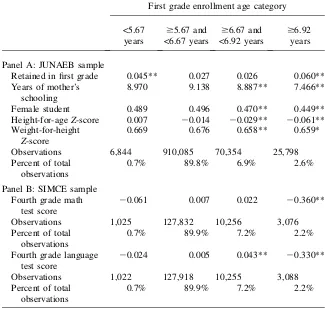
In the JUNAEB sample, the average student entered first grade at age 6.3, and 2.8 percent of students are retained in the first grade (Table 1). The latest possible enroll-ment cutoff is July 1, implying a minimum enrollenroll-ment age of 5.67. Less than 1 per-cent of the sample violates this cutoff by enrolling earlier (Table 2). Some schools use cutoffs as early as April 1, implying a minimum enrollment age of 5.92 years and a maximum of 6.92. Table 2, Panel A shows that only 2.6 percent of students delay enrollment past 6.92 years of age.
Students who voluntarily delay enrollment past 6.92 years have greater probabil-ities of being retained in the first grade and much lower test scores (Table 2). The same children that delay enrollment also have less-educated mothers, worse anthro-pometric indicators, and are more likely to be male. They also, presumably, differ on unobservable dimensions that affect outcomes, thus biasing enrollment age effects based on Equation 1.
IV. Effects on First Grade Retention
A. Results
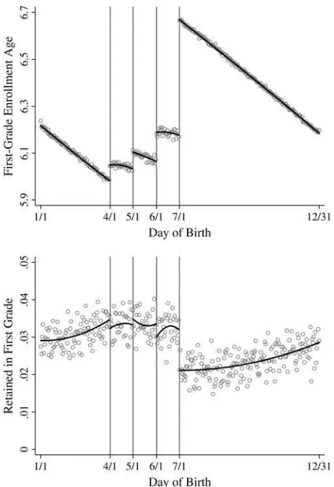
The top panel of Figure 1 graphs first grade enrollment age against day of birth. The points show means within day-of-birth cells, and they reveal sharp increases in
18. The adjustment models the probability a respondent will correctly answer a test score item as a func-tion of the student’s latent ability and the item’s difficulty. This scaling sharpens the correspondence be-tween a one-point test score increase and a one-unit increase in a student’s cognitive skills (Yamamoto and Kulick 1999).
enrollment age on the first days of April, May, June, and July. The first three cut-offs show differences of less than 0.1 years, and July 1 indicates a difference of half a year. The solid line plots fitted values from the piecewise quadratic spline in Equation 3. The bottom panel of Figure 1 examines whether sharp variation in enrollment age near the cutoffs is accompanied by changes in first grade reten-tion (as in the reduced form in Equareten-tion 2). Students born on July 1 and thereafter have a lower probability of retention, by approximately one percentage point—a substantial effect given the full sample mean retention rate of 2.8 percent.
Table 2
Retained in first grade 0.045** 0.027 0.026 0.060**
Years of mother’s schooling
8.970 9.138 8.887** 7.466**
Female student 0.489 0.496 0.470** 0.449**
Height-for-ageZ-score 0.007 20.014 20.029** 20.061** Weight-for-height
20.061 0.007 0.022 20.360**
Observations 1,025 127,832 10,256 3,076
20.024 0.005 0.043** 20.330**
Observations 1,022 127,918 10,255 3,088
Percent of total observations
0.7% 89.9% 7.2% 2.2%
Notes: Each row reports variable means by four enrollment age categories. ** (*) indicates that a row mean is statistically different from the mean of students in the second category (enrollment at$5.67 and <6.67 years) at 1 percent (5 percent). Hypothesis tests account for clustering of students within schools.
Tables 3 and 4 summarize estimates from first-stage, reduced-form, and TSLS regressions that mirror Figure 1.21The first-stage estimates (Table 3, Columns 1 to 3) confirm that enrollment age increases around enrollment cutoffs, particularly July 1.
Figure 1
Day of Birth, First grade Enrollment Age, and First grade Retention Source: JUNAEB sample.
Note: The dots are mean values of they-axis variable within each day of birth. The solid lines are fitted values from a piecewise quadratic of day of birth (see text for details).
Table 3
Effects of enrollment age on first grade retention (first-stage and reduced-form regressions)
Dependent variable: First grade enrollment age Dependent variable: Retained in first grade
(1) (2) (3) (4) (5) (6)
D1(born on or after April 1) 0.069** 0.067** 0.066** 20.0024 20.0028 20.0036*
(0.004) (0.004) (0.004) (0.0017) (0.0017) (0.0016)
D2(born on or after May 1) 0.071** 0.067** 0.067** 0.0016 0.0023 0.0022
(0.007) (0.007) (0.007) (0.0027) (0.0028) (0.0029)
D3(born on or after June 1) 0.124** 0.118** 0.118** 20.0035 20.0032 20.0032
(0.009) (0.008) (0.008) (0.0022) (0.0022) (0.0023)
D4(born on or after July 1) 0.493** 0.467** 0.467** 20.0107** 20.0103** 20.0101**
(0.007) (0.005) (0.005) (0.0018) (0.0017) (0.0019)
R2 0.252 0.445 0.447 0.001 0.002 0.015
(continued)
McEwan
and
Shapiro
Table 3(continued)
Dependent variable: First grade enrollment age Dependent variable: Retained in first grade
(1) (2) (3) (4) (5) (6)
Fstatistic 1,560 2,157 2,157
p-value [<0.001] [<0.001] [<0.001]
Piecewise quadratic of B Yes Yes Yes Yes Yes Yes
Birth-year dummy variables No Yes Yes No Yes Yes
Day-of-week dummy variables No Yes Yes No Yes Yes
Holiday dummy variable No Yes Yes No Yes Yes
Student control variables No No Yes No No Yes
Source: JUNAEB sample.
Notes: The number of observations in each regression is 1,013,081. ** (*) indicates statistical significance at 1 percent (5 percent). Robust standard errors, adjusted for clustering within 366 day-of-birth cells, appear in parentheses. TheF-statistic corresponds to a test of the null hypothesis that the four instruments,D1toD4, are jointly zero (p-values in brackets). Student control variables include Female, Height-for-ageZ-score, Weight-for-heightZ-score, and dummy variables indicating discrete cat-egories of Mother’s schooling. All regressions include a constant.
The
Journal
of
Human
Each instrument has larget-statistics and the F-statistic on the joint significance of the instruments is 1,560. Coefficients change little with inclusion of controls. The reduced-form estimates confirm, in the vicinity of the July 1 cutoff, a statistically
Table 4
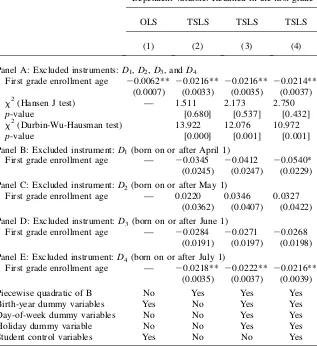
Effects of enrollment age on first grade retention (TSLS regressions)
Dependent variable: Retained in the first grade
OLS TSLS TSLS TSLS
(1) (2) (3) (4)
Panel A: Excluded instruments:D1,D2,D3, andD4
First grade enrollment age 20.0062** 20.0216** 20.0216** 20.0214** (0.0007) (0.0033) (0.0035) (0.0037)
x2(Hansen J test) — 1.511 2.173 2.750
p-value [0.680] [0.537] [0.432]
x2(Durbin-Wu-Hausman test) 13.922 12.076 10.972
p-value [0.000] [0.001] [0.001]
Panel B: Excluded instrument:D1(born on or after April 1)
First grade enrollment age — 20.0345 20.0412 20.0540* (0.0245) (0.0247) (0.0229) Panel C: Excluded instrument:D2(born on or after May 1)
First grade enrollment age — 0.0220 0.0346 0.0327
(0.0362) (0.0407) (0.0422) Panel D: Excluded instrument:D3(born on or after June 1)
First grade enrollment age — 20.0284 20.0271 20.0268 (0.0191) (0.0197) (0.0198) Panel E: Excluded instrument:D4(born on or after July 1)
First grade enrollment age — 20.0218** 20.0222** 20.0216** (0.0035) (0.0037) (0.0039)
Piecewise quadratic of B No Yes Yes Yes
Birth-year dummy variables Yes No Yes Yes
Day-of-week dummy variables No No Yes Yes
Holiday dummy variable No No Yes Yes
Student control variables Yes No No Yes
Source: JUNAEB sample.
Notes: The number of observations in each regression is 1,013,081. ** (*) indicates statistical significance at 1 percent (5 percent). Robust standard errors, adjusted for clustering within 366 day-of-birth cells, are in parentheses. Cells in Columns 2, 3, and 4 report the coefficient on First grade enrollment age from sep-arate TSLS regressions that use different excluded instruments (see panel headings) and controls (see bot-tom of table). Student control variables include Female, Height-for-age Z-score, Weight-for-height Z-score, and dummy variables indicating discrete categories of Mother’s schooling. All regressions in-clude a constant.
significant decline of around one percentage point in the retention probability (see Columns 4 to 6).
Table 4, Panel A reports TSLS estimates that exploit enrollment age variation at all four cutoffs to estimate causal effects. In Column 1, an OLS estimate with student controls suggests that increasing enrollment age has a negative but small effect on the probability of being retained in the first grade. Descriptive statistics implied that such an estimate would be biased because disadvantaged students—more likely to be retained—voluntarily delay enrollment. In fact, the estimates from TSLS specifica-tions are over three times the magnitude of OLS estimates and stable across speci-fications. They suggest that a one-year delay in enrollment lowers the probability of repeating first grade by 2.1 percentage points. In the over-identified regression, HansenJtests producep-values above 0.4, providing no evidence against the instru-ments’ validity. Durbin-Wu-Hausman tests reject the null hypothesis that enrollment age is exogenous and justify using TSLS (though having a million observations makes a large test statistic more likely).
Panels B to E report four exactly identified models that use sharp variation around each cutoff as a single excluded instrument. The estimates that rely on variation around April 1 and June 1 have negative signs, with larger magnitude than previous results and imprecise estimates. The estimates relying on variation around May 1 have positive signs and larger standard errors. Given the strength of the July 1 instru-ment, estimates in Panel E are very similar to estimates in Panel A.
B. Evidence of Birth Timing
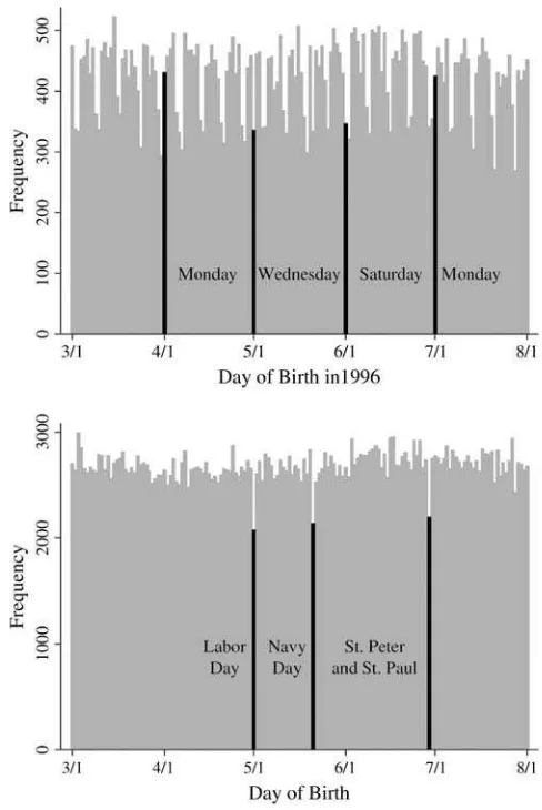
In Chile, as in many countries, scheduled births cause the frequency of birthdate distributions to decline on weekends and holidays (Dickert-Conlin and Chandra 1999). The top panel of Figure 2 illustrates the weekend dip among sample chil-dren born in 1996. This dip is not evident among a pooled sample of all birth years (bottom panel), though births noticeably decline on three national holidays, two of which are close to enrollment cutoffs. In the sample data, mothers of Sunday births have 0.18 fewer years of schooling, relative to Mondays, and mothers of hol-iday births have 0.07 fewer years, relative to other days (McEwan and Shapiro 2006).
A first, less pressing concern is that enrollment cutoffs coincidentally fall near weekends and holidays, as Figure 2 shows happened in 1996. Even in the absence of strategic birth timing, such coincidence could introduce correlation between en-rollment age and mother’s schooling (or unobservables). Despite these concerns, controlling for day-of-week and holiday indicators in regressions barely changes estimates (Tables 3 and 4).
services and knowledge of school policies. Birth timing of this kind would bias effects on grade retention toward zero, presuming that families born before cutoffs have spuriously low retention rates. Our estimates suggest large impacts despite this potential bias.
Figure 2
Day of Birth Histograms, in 1996 and Pooled across Birth Years Source: JUNAEB sample.
Note: The top panel includes children born in 1996, and the bottom panel includes all children. The three labeled bars indicate holidays on May 1 (Labor Day), May 21 (Navy Day), and June 29 (St. Peter and St. Paul).
Table 5
Effects of enrollment age on first grade retention (alternate TSLS regressions)
Excluded instruments Specification of f(B)
Dependent variable
Model Sample [observations] Retained in first grade
1 Full [1,013,081] D1-D4 Quadratic 20.0214** (0.0037)
2 Full [1,013,081] D1-D4 Linear 20.0267** (0.0027)
3 Full [1,013,081] D1-D4 Cubic 20.0210** (0.0052)
4 6/17–7/14 [76,617] D4 None 20.0240** (0.0027)
5 6/17–6/23 and 7/8–7/14 [38,303] D4 None 20.0273** (0.0038)
6 Regions 3 and 7–10 [347,632] D1-D4 Quadratic 20.0216** (0.0070)
7 Full [1,013,081] QOB None 20.0218** (0.0012)
8 Girls [499,027] D1-D4 Quadratic 20.0187** (0.0055)
9 Boys [514,054] D1-D4 Quadratic 20.0241** (0.0050)
By mother’s schooling
10 0–7 years [260,800] D1-D4 Quadratic 20.0233* (0.0102)
11 8 years [167,734] D1-D4 Quadratic 20.0372** (0.0091)
12 9–11 years [224,456] D1-D4 Quadratic 20.0171** (0.0060)
13 12 years [273,083] D1-D4 Quadratic 20.0160** (0.0047)
14 Any postsecondary [87,008] D1-D4 Quadratic 20.0179** (0.0063)
Source: JUNAEB sample.
Notes: ** (*) indicates statistical significance at 1 percent (5 percent). Robust standard errors, adjusted for clustering within day-of-birth cells, are in parentheses. The baseline specification (Model 1) reports the coefficient on First grade enrollment age from the TSLS regression in Table 4, Panel A, Column 4. Additional rows report the coefficient from modified samples and specifications. In Model 7, QOB indicates three dummies for the second, third, and fourth quarters of birth.
The
Journal
of
Human
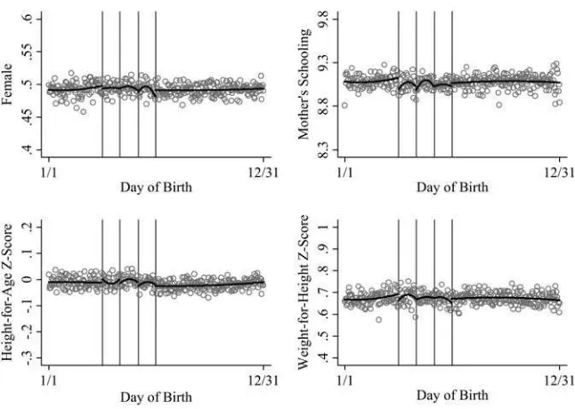
As an additional check, we assess whether students’ characteristics vary sharply near enrollment cutoffs.22Figure 3 plots the mean values of student characteristics within day-of-birth cells, revealing no large breaks near cutoffs and even little sea-sonality. To confirm these findings, we estimate four variants of Equation 2, using student attributes as dependent variables. Of 16 coefficients on the four Dj, only
two are statistically significant (D1 for mother’s schooling, and D4 for female),
though they have small magnitude.23
Figure 3
Testing Smoothness of Baseline Variables across Enrollment Cutoffs Source: JUNAEB sample.
Note: The dots are mean values of they-axis variable within each day of birth. The solid lines are fitted values from a piecewise quadratic of day of birth (see text for details). The y-axis of continuous variables is scaled to about half a standard deviation. The four vertical lines in each panel are placed at April 1, May 1, June 1, and July 1.
22. We expect student height and weight to differ sharply across early and late-entering students, given a difference in age when the measurement it taken at the beginning of first grade (the results are available from the authors). However, we do not anticipate sharp differences in age-adjustedZ-scores, unless parents on either side of cutoffs respond to assigned enrollment dates by altering investments in nutrition. 23. McEwan and Shapiro (2006) report the complete estimates. Results are also insensitive to including day-of-week and holiday indicators.
C. Robustness and Heterogeneous Effects
The first row of Table 5 (Model 1) reports the original TSLS estimate of b1 from
Table 4, Panel A, Column 4. Subsequent rows report estimates from varying samples and specifications. Models 2 and 3 vary the specification of f(B) in the first- and second-stage regressions. A piecewise linear specification yields a more negative point estimate of20.027, while a piecewise cubic produces an estimate very similar to the baseline. Model 4 limits the sample to children born in two-week intervals on either side of the July 1 cutoff, diminishing reliance on arbitrary functional form assumptions and data far from the cutoff (Chay, McEwan, and Urquiola 2005). The point estimate of20.024 is very similar. Model 5 adds an additional sample restric-tion to Model 4, dropping students in one-weekintervals on either side, since precise timing is most likely to occur in these days. The point estimate becomes only slightly more negative. Model 6 reestimates the baseline specification using five of Chile’s 13 regions with less sample selection,24yielding a similar point estimate to the baseline.
Model 7 assesses whether simpler, quarter-of-birth instruments and no controls for smooth functions of birth dates in TSLS regressions, in the spirit of Angrist and Krueger (1991), can obtain the same results. The usual concern is that seasonality in conception creates correlations between quarter of birth and unexplained variation in outcomes (Bound, Jaeger, Baker 1995; Bound and Jaeger 2000). Figure 3 was not consistent with this concern, given the flat relationship between birth date and com-mon correlates of outcomes. In fact, the point estimate of the simpler model is nearly identical to the baseline, suggesting that in Chilean data, coarser birth date measures can be a useful source of identification.
Finally, we estimate the baseline specification in subsamples to assess how effects on retention vary across different children. Reductions in first grade retention are slightly larger for boys (Models 8-9), and for children whose mothers have relatively less schooling (models 10-14). However, boys and children of less-educated mothers also have higher baseline retention rates. For example, in the lowest and highest groups of mother’s schooling defined in Table 5, the mean first grade retention is 0.053 and 0.001, respectively.25
V. Effects on Test Scores
A. Results
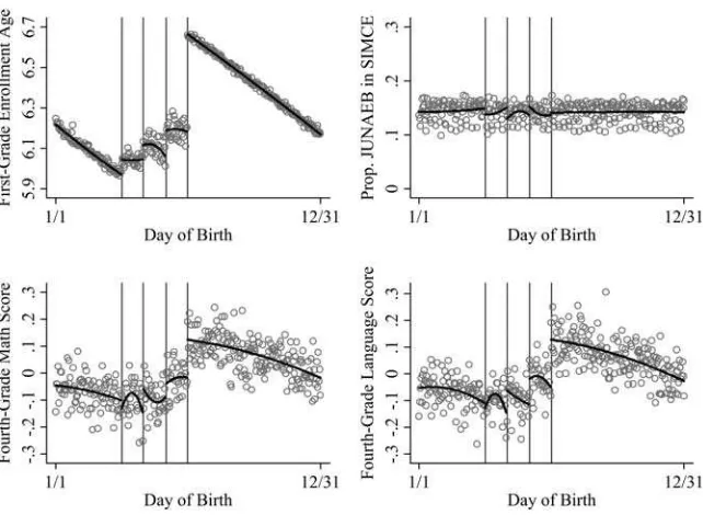
In the fourth grade SIMCE sample, Figure 4 (top-left) shows that first grade enroll-ment age increases sharply at cutoffs, as in Figure 1, but with slightly more noise. The estimated breaks in first-stage regressions are similar those in the full sam-ple—0.48 years on July 1, and 0.07 to 0.13 years at earlier cutoffs.26The lower
24. The subsample includes 84 (87) percent of schools (students) (McEwan and Shapiro 2006). 25. In subsamples of boys and girls, the first grade retention rates are 0.030 and 0.025, respectively. Elder and Lubotsky (2006) find similar patterns across socioeconomic quartiles in U.S. data.
panels of Figure 4 illustrate the reduced-form discontinuity analysis for fourth grade math and language test scores. The unsmoothed means and fitted values suggest changes of 0.15 to 0.2 standard deviations in test scores at the July 1 cutoff. Table 6 reports TSLS estimates for fourth grade math and language test scores (Panel A, Model 1) that rely on sharp variation in enrollment age at all cutoffs. The reported estimates include a full set of controls (see table note). They suggest that delaying enrollment by one year increases fourth grade test scores by a statistically-significant 0.29 standard deviations in math and 0.38 standard deviations in language. Birth his-tograms and comparisons of student variables across cutoffs show no evidence of birth timing (McEwan and Shapiro 2006).
In the TIMSS sample, the first-stage estimates show an increased age of 0.4 years for children born on July 1, with at-statistic of 3.9 in the fully specified model. Esti-mates of breaks at earlier cutoffs have statistically insignificant coefficients—despite magnitudes consistent with other samples—andF-statistics on joint significance do not exceed 13 (McEwan and Shapiro 2006). In TSLS estimates for the eighth grade data, we use only a single excluded instrument (D4) in an exactly identified version Figure 4
Day of Birth, First grade Enrollment Age, and Fourth grade Test Scores Source: SIMCE sample.
Note: The dots are mean values of they-axis variable within each day of birth. The solid lines are fitted values from a piecewise quadratic of day of birth (see text for details). The four vertical lines in each panel are placed at April 1, May 1, June 1, and July 1.
Table 6
Effects of enrollment age on fourth- and eighth grade test scores (TSLS regressions)
Sample [observations for math; observations for
language or science]
Excluded instruments
Specification of f(B)
Dependent variable
Model Math test Language test
Panel A: Fourth grade SIMCE sample
1 Full [142,189;142,283] D1-D4 Quadratic 0.2864** (0.0472) 0.3812** (0.0574)
2 Full [142,189;142,283] D1-D4 Linear 0.2871** (0.0379) 0.3466** (0.0448)
3 Full [142,189;142,283] D1-D4 Cubic 0.2465** (0.0660) 0.3413** (0.0770)
4 6/17–7/14 [10,490;10,469] D4 None 0.2897** (0.0433) 0.3375** (0.0464)
5 6/17–6/23 and 7/8–7/14 [5,258;5,237] D4 None 0.2931** (0.0576) 0.3474** (0.0584)
6 Regions 3 and 7–10 [48,535;48,609] D1-D4 Quadratic 0.2259* (0.0944) 0.2801** (0.0949)
7 Full [142,189,142,283] QOB None 0.3911** (0.0163) 0.3891** (0.0155)
8 Girls [70,466;70,537] D1-D4 Quadratic 0.2455** (0.0706) 0.3172** (0.0676)
9 Boys [71,723;71,746] D1-D4 Quadratic 0.326** (0.0870) 0.4354** (0.0804)
By mother’s schooling
10 0–7 years [34,321;34,405] D1-D4 Quadratic 0.1607 (0.1055) 0.4222** (0.1095)
11 8 years [24,918;24,951] D1-D4 Quadratic 0.5649** (0.1013) 0.3941** (0.1094)
The
Journal
of
Human
12 9–11 years [32,258;32,225] D1-D4 Quadratic 0.3406** (0.1015) 0.4234** (0.1349)
13 12 years [38,867;38,870] D1-D4 Quadratic 0.1919 (0.1068) 0.2424* (0.1112)
14 Any postsecondary [11,825;11,832] D1-D4 Quadratic 0.1431 (0.1935) 0.5200** (0.1827)
Panel B: Eighth grade TIMSS sample Math test Science test
1 Full [5,582; 5,582] D4 Quadratic 0.4282 (0.2795) 0.7198* (0.2860)
2 Full [5,582; 5,582] D4 Linear 0.1581 (0.1904) 0.8456** (0.2128)
3 Full [5,582; 5,582] D4 Cubic 0.2564 (0.2889) 0.3029 (0.2601)
4 6/17–7/14 [389; 389] D4 None 20.0497 (0.7482) 0.3687 (0.5660)
5 Full [5,582; 5,582] QOB None 0.2508* (0.1730) 0.4512** (0.1742)
Source: SIMCE and TIMSS samples.
Notes: ** (*) indicates statistical significance at 1 percent (5 percent). Robust standard errors, adjusted for clustering within 366 day-of-birth cells, are in parentheses. Panel A, Model 1 reports coefficients on First grade enrollment age from TSLS regressions, in the SIMCE sample, with controls for a piecewise quadratic of B, day-of-week dummies, a holiday dummy, Female, Height-for-ageZ-score, Weight-for-heightZ-score, dummy variables indicating discrete categories of Mother’s schooling, and a constant. Panel B, Model 1 reports coefficients on Enrollment age from TSLS regressions, in the TIMSS sample, with controls for a piecewise quadratic of B, day-of-week dummies, a holiday dummy, the TIMSS variables described in the text, and a constant. TIMSS sample weights are applied. QOB indicates three dummies for the second, third, and fourth quarters of birth.
McEwan
and
Shapiro
of Equations 4 and 5. In Table 6 (Panel B, Model 1), the full TSLS estimates show that a one-year increase in enrollment age increases eighth grade test scores by 0.43 standard deviations in math and 0.72 standard deviations in science. The former co-efficient is statistically insignificant at 5 percent, though itst-statistic exceeds 1.5.
Interpretation of test score effects requires several caveats. First, student drop-outs in upper grades could introduce sample selection bias if they occur near enrollment cutoffs. However, enrollment rates are above 98 percent in age groups between seven and 13 (McEwan, Forthcoming). The top-right panel of Figure 4 and other regression estimates (available from the authors) confirm that the proportion of first graders matched to fourth grade records does not vary sharply around enrollment cutoff dates.
Second, both test score samples include retained students. Grade retention and the concomitant reshuffling of first grade cohorts across upper-primary grades could un-dermine the identification strategy. Consider the sample of fourth graders in 2002. Over 90 percent did not repeat a grade, having entered first grade in 1999 (Table 1). Eight percent were retained, having begun first grade in 1998. They ‘‘replace’’ a portion of retained 1999 entrants who will not reach fourth grade until at least 2003.
Our evidence suggests that repeaters are disproportionately students born to the left of enrollment cutoffs, perhaps creating unobserved differences between students on either side of cutoffs. These differences could undermine identifying Assumption 6. However, if the two compositional effects cancel out close to enrollment cutoffs, this effect will not bias estimates. In practical terms, the 2002 sample would add repeaters from the 1998 cohort of first graders, ‘‘replacing’’ repeaters from the 1999 cohort that have yet to reach the fourth grade. The two groups are perhaps sim-ilar in size and simsim-ilar in unobserved characteristics associated with grade repetition, partly confirmed by the absence of differences in observed characteristics across breaks.
Third, the grade-specific samples are each dominated by two birth year cohorts (1992 and 1993, in the case of fourth graders). Students to the right of the July 1 cutoff, who delay enrollment, are drawn from the older cohort. To identify enroll-ment age effects at discontinuities in such sample, we do not include a birth year dummy. The absence of sharp differences in observed student characteristics, and the replication of test score effects across two samples, provides a measure of con-fidence that our estimates are not explained by coincidental effects across birth year cohorts.
B. Robustness and Heterogeneity
In the fourth grade sample, a one-year increase in enrollment age improves boys’ test scores by about one-third more than girls. Some evidence indicates that math effects are larger among children of less-educated mothers, although the pattern of effects is not monotone, and there is no such pattern for language effects.
VI. Discussion
A. Homogeneous Results
Enrollment age effects, though causal, operate through three pathways. Students who delay enrollment will be older when schools evaluate them. In support of this age-at-test effect, Elder and Lubotsky (2006) find large effects of ‘‘enrollment age’’ on age-at-test scores in the Fall of kindergarten, before schools could plausibly contribute to learn-ing (also see Datar 2006). Such effects might fade over time, since a year of matu-ration represents more learning among young children than among adolescents (Bedard and Dhuey 2006; Elder and Lubotsky 2006).
Second, delayed enrollment increases a student’s absolute age of enrollment. Older students acquire cognitive, social, linguistic, or physical abilities—often termed ‘‘school readiness’’—that may allow them to learn more in school than youn-ger children do (see Stipek 2002).
Third, delayed enrollment increases a student’s age of enrollment relative to her classmates. In Chile, a plausible relative age effect operates through primary school admissions, since some publicly-funded private schools select students from admis-sions queues (Gauri 1998). If maturation gives older students an advantage when they apply, and maturation affects factors considered in school admissions, then pri-vate schools with a queue may select disproportionately older children. School per-sonnel also could introduce differences in the educational inputs that relatively older and younger children receive in primary grades. Grouping students by ability (‘‘tracking’’) may place older children in higher ability groups (Bedard and Dhuey 2006), but also could disproportionately allocate compensatory programs like reme-dial tutoring toward lower-achieving, relatively young students (Chay, McEwan, and Urquiola 2005).
Our results cohere more with enrollment age effects than with age-at-test effects. Elder and Lubotsky (2006) find declining enrollment age effects in upper grades, interpreted as evidence of dominant age-at-test effects. Bedard and Dhuey (2006) find more persistent effects that decline slightly by eighth grade, and argue that age-at-test effects cannot fully explain results. Our findings on test scores show per-sistent or increasing effects, conper-sistent with either absolute or relative enrollment age effects. Because of prevalent school choice in Chile (McEwan and Carnoy 2000), we suspect that that relative age effects play some role. Correspondingly, Chilean results may have limited implications for countries with less school choice.
B. Heterogeneous Results
A one-year delay produces larger decreases in retention probabilities among students with less-educated mothers, though heterogeneity in test score effects is inconsistent. One explanation for the pattern of retention effects focuses on retention as a binary
indicator of a student’s unobserved achievement at the end of first grade. Suppose we have populations of high- and low- achieving students identified by superscripts H andL, respectively. Each student has unobserved achievement ai, with aHi ;N
ðmH;s
L,mH. Retentionriindicates that a student failed
to meet a low achievement thresholda: ri¼1fai,ag where1{}is the indicator
function and a,minfmL;mHg. Suppose that delaying enrollment improves the
achievement of all students by the scalarf. IfFp()denotes the cumulative distribu-tion funcdistribu-tion andfp()denotes the density function both for populationp, then the change in retention rate due to delayed enrollment for populationpis
Z a
a2f
fpðaÞda¼FpðaÞ2Fpða2fÞ
A normal density function has positive slope for values below its mean. Since
mL,mH, since both distributions are normal with the same variance, and since
a,minfmL;mHg, we obtain
FLðaÞ 2FLða2fÞ.FHðaÞ2FHða2fÞ ð7Þ
The inequality shows that delayed enrollment will affect the retention of low-achieving students—perhaps those with less-educated mothers—more than that of high-achieving students, even if effects on unobserved first grade achievement are homo-geneous.
Among boys, delaying enrollment produces consistently larger decreases in reten-tion and larger increases in test scores. One explanareten-tion is that similarly aged boys and girls possess different levels of school readiness. In particular, similarly aged boys might be less mature or ‘‘ready’’ for schooling. Some psychologists believe that increased readiness—the result of delayed enrollment and maturation—only improves children’s later schooling outcomes until a threshold level of readiness is reached (Stipek 2002). If more girls already exceed this threshold at a given age than boys do, then the marginal effect of an additional one-year delay would be lower among girls.
VII. Conclusions and Policy Implications
An exogenous one-year delay in first grade enrollment decreases the probability of first grade retention by about two percentage points, relative to a base-line of 2.8 percent, and increases fourth- and eighth grade test scores by 0.3 or more standard deviations. The persistent effects suggest that absolute or relative enroll-ment age, rather than age-at-test, explain these results.
school (Elder and Lubotsky 2006; Stipek 2002). Second, if relative age effects dom-inate, then moving cutoff dates earlier would merely redistribute achievement among students without increasing mean test scores. Third, if absolute age effects dominate, then raising mean enrollment age would increase mean test scores by improving stu-dents’ readiness for school.
The uncertain benefits of uniformly increasing the mean enrollment age must be weighed against potentially large costs: childcare, shortened work careers, and lower attainment. The relatively low incidence ofvoluntaryenrollment delays, at least in Chile, suggests that the benefits of delays outweigh costs for only a small proportion of families. Among such families, voluntary delays can be viewed as a rational and tacit investment in the human capital of disadvantaged children.27Much evidence from developing countries suggests, for example, that families voluntarily delay en-rollment of malnourished and stunted children (Alderman, Hoddinott, and Kinsey 2006; Glewwe and Jacoby 1995; Glewwe, Jacoby, and King 1999; McEwan 2006; Partnership for Child Development 1999). Instead of permitting tacit investments through voluntary delays—or mandating delays for all children—policymakers might instead consider direct, targeted investments in children’s school readiness, such as early childhood nutrition (Rawlings and Rubio 2005) and preschool (Berlinski, Galiani, and Gertler 2006; Gormley and Gayer 2005).
References
Alderman, Harold, John Hoddinott, and Bill H. Kinsey. 2006. ‘‘Long term Consequences of Early Childhood Malnutrition.’’Oxford Economic Papers58(3):450–74.
Angrist, Joshua D., and Guido W. Imbens. 1995. ‘‘Two-Stage Least Squares Estimation of Average Causal Effects in Models with Variable Treatment Intensity.’’Journal of the American Statistical Association90(430):431–42.
Angrist, Joshua D., and Alan B. Krueger. 1991. ‘‘Does Compulsory School Attendance Affect Schooling and Earnings?’’Quarterly Journal of Economics106(4):979–1014.
Bedard, Kelly, and Elizabeth Dhuey. 2006. ‘‘The Persistence of Early Childhood Maturity: International Evidence of Long-Run Age Effects.’’Quarterly Journal of Economics 121(4):1437–72.
Beliza´n, Jose´ M., Fernando Althabe, Fernando C. Barros, and Sophie Alexander. 1999. ‘‘Rates and Implications of Caesarean Sections in Latin America: Ecological Study.’’BMJ 319:1397–1400.
Berlinski, Samuel, and Sebastian Galiani. 2007. ‘‘The Effect of a Large Expansion of PrePrimary School Facilities on Preschool Attendance and Maternal Employment.’’Labour Economics.Forthcoming.
Berlinski, Samuel, Sebastian Galiani, and Paul Gertler. 2006. ‘‘The Effect of Pre-Primary Education on Primary School Performance.’’ Working Paper W06/04. London: The Institute for Fiscal Studies.
27. Glewwe and Jacoby (1995) formalize this intuition by adding to a dynamic human capital model the assumption that some children are less ready for school at a specified enrollment age, and that voluntary delays increase readiness. They further assume that readiness at enrollment increases subsequent earnings, providing the necessary scope for some families to delay enrollment voluntarily, despite the associated costs. Delayed enrollment in poor settings also could reflect credit constraints, if families are unable to fi-nance the direct or indirect costs of primary school (Bommier and Lambert 2000; Glewwe and Jacoby 1995).
Bommier, Antoine, and Sylvie Lambert. 2000. ‘‘Education Demand and Age at School Enrollment in Tanzania.’’Journal of Human Resources35(1):177–203.
Bound, John, and David A. Jaeger. 2000. ‘‘Do Compulsory Attendance Laws Alone Explain the Association Between Earnings and Quarter of Birth?’’ InResearch in Labor Economics: Worker Well-Being,ed. Solomon W. Polacheck, 83–108. New York: JAI. Bound, John, David A. Jaeger, and Regina M. Baker. 1995. ‘‘Problems With Instrumental
Variables Estimation When the Correlation Between the Instruments and the Endogenous Explanatory Variable Is Weak.’’Journal of the American Statistical Association 90(430):443–50.
Cascio, Elizabeth. 2006. ‘‘Public Preschool and Maternal Labor Supply: Evidence from the Introduction of Kindergartens into American Public Schools.’’ Working Paper 12179. Cambridge: National Bureau of Economic Research.
Cascio, Elizabeth U., and Ethan G. Lewis. 2006. ‘‘Schooling and the AFQT: Evidence from School Entry Laws.’’Journal of Human Resources41(2):294–318.
Chay, Kenneth Y., Patrick J. McEwan, and Miguel Urquiola. 2005. ‘‘The Central Role of Noise in Evaluating Interventions That Use Test Scores to Rank Schools.’’American Economic Review95(4):1237–58.
Datar, Ashlesha. 2006. ‘‘Does Delaying Kindergarten Entrance Give Children a Head Start?’’ Economics of Education Review25(1):43–62.
Dickert-Conlin, Stacy, and Amitabh Chandra. 1999. ‘‘Taxes and the Timing of Births.’’ Journal of Political Economy107(1):161–77.
Elder, Todd E., and Darren H. Lubotsky. 2006. ‘‘Kindergarten Entrance Age and Children’s Achievement: Impacts of State Policies, Family Background, and Peers.’’ University of Illinois at Urbana-Champaign. Unpublished.
Fredriksson, Peter, and Bjo¨rn O¨ ckert. 2005. ‘‘Is Early Learning Really More Productive? The Effect of School Starting Age on School and Labor Market Performance?’’ Uppsala University. Unpublished.
Gauri, Varun. 1998.School Choice in Chile.Pittsburgh: University of Pittsburgh Press. Gelbach, Jonah B. 2002. ‘‘Public Schooling for Young Children and Maternal Labor Supply.’’
American Economic Review92(1):307–22.
Glewwe, Paul, and Hanan G. Jacoby. 1995. ‘‘An Economic Analysis of Delayed Primary School Enrollment in a Low Income Country: The Role of Early Childhood Nutrition.’’ Review of Economics and Statistics77(1):156–69.
Glewwe, Paul, Hanan G. Jacoby, and Elizabeth M. King. 2001. ‘‘Early Childhood Nutrition and Academic Achievement: A Longitudinal Analysis.’’Journal of Public Economics 81(3):345–68.
Gormley, William T., and Ted Gayer. 2005. ‘‘Promoting School Readiness in Oklahoma: An Evaluation of Tulsa’s PreK Program.’’Journal of Human Resources40(3):533–58. Hsieh, Chang-Tai, and Miguel Urquiola. 2006. ‘‘The Effects of Generalized School Choice on
Achievement and Stratification: Evidence from Chile’s Voucher System.’’Journal of Public Economics90(8-9):1477–1503.
Lee, David S. Forthcoming. ‘‘Randomized Experiments from Non-Random Selection in U.S. House Elections.Journal of Econometrics.
Lee, David S., and David Card. Forthcoming. ‘‘Regression Discontinuity Inference with Specification Error.’’Journal of Econometrics.
Lemieux, Thomas, and Kevin Milligan. 2005. ‘‘Incentive Effects of Social Assistance: A Regression Discontinuity Approach.’’ University of British Columbia. Unpublished. McCrary, Justin. Forthcoming. ‘‘Manipulation of the Running Variable in the Regression
McCrary, Justin, and Heather Royer. 2006. ‘‘The Effect of Maternal Education on Fertility and Infant Health: Evidence from School Entry Laws Using Exact Date of Birth.’’ University of Michigan. Unpublished.
McEwan, Patrick J. 2006. ‘‘Delayed Primary School Enrollment in Eight Latin American Countries.’’ Wellesley College. Unpublished.
———. Forthcoming. ‘‘Can Schools Reduce the Indigenous Test Score Gap? Evidence from Chile.’’Journal of Development Studies.
McEwan, Patrick J., and Martin Carnoy. 2000. ‘‘The Effectiveness and Efficiency of Private Schools in Chile’s Voucher System.’’Educational Evaluation and Policy Analysis 22(3):213–39.
McEwan, Patrick J., and Joseph S. Shapiro. 2006. ‘‘The Consequences of Delayed Primary School Enrollment in a Developing Country.’’ Wellesley College and LSE. Unpublished. Murray, Susan F. 2000. ‘‘Relation between Private Health Insurance and High Rates of
Caesarean Section in Chile: Qualitative and Quantitative Study.’’BMJ321:1501–1505. Partnership for Child Development. 1999. ‘‘Short Stature and the Age of Enrolment in
Primary School: Studies in Two African Countries.’’Social Science and Medicine 48(5):675–82.
Rawlings, Laura B., and Gloria M. Rubio. 2005. ‘‘Evaluating the Impact of Conditional Cash Transfers.’’World Bank Research Observer20(1):29–55.
Repu´blica de Chile. 1992. ‘‘Determina Fecha en Que Reconoce Cumplimento de Edad de Ingreso a la Educacio´n Parvularia Segundo Nivel de Transicio´n y Educacio´n Ba´sica.’’ Santiago: Repu´blica de Chile, Ministerio de Educacio´n.
Stipek, Deborah. 2002. ‘‘At What Age Should Children Enter Kindergarten? A Question for Policy Makers and Parents.’’Social Policy Report16(2):3–17.
UNESCO. 2007. ‘‘Length and Starting Age of Compulsory Education for Schools Years 1998/1999 to 2004/2005.’’ UNESCO Institute for Statistics.
Urquiola, Miguel, and Valentina Caldero´n. 2006. ‘‘Apples and Oranges: Educational Enrollment and Attainment across Countries in Latin America and the Caribbean.’’ International Journal of Educational Development26(6):572–90.
van der Klaauw, Wilbert. 2002. ‘‘Estimating the Effect of Financial Aid Offers on College Enrollment: A Regression-Discontinuity Approach.’’International Economic Review 43(4):1249–86.
Yamamoto, Kentaro, and Edward Kulik. 2000. ‘‘Scaling Methodology and Procedures for the TIMSS Mathematics and Science Scales.’’ In TIMSS1999 Technical Report,ed. Michael O. Martin, Kelvin D. Gregory, and Steven E. Stemler, 259–77. Boston: International Study Center, Boston College.