Manajemen | Fakultas Ekonomi Universitas Maritim Raja Ali Haji 750.full

(1)

T H E J O U R N A L O F H U M A N R E S O U R C E S • 46 • 4

Estimates of Year-to-Year Volatility

in Earnings and in Household

Incomes from Administrative,

Survey, and Matched Data

Molly Dahl

Thomas DeLeire

Jonathan A. Schwabish

A B S T R A C T

We document trends in the volatility in earnings and household incomes between 1985 and 2005 in three different data sources: administrative earnings records, the Survey of Income and Program Participation (SIPP) matched to administrative earnings records, and SIPP survey data. In all data sources, we find a substantial amount of year-to-year volatility in workers’ earnings and household incomes. In the data sources that contain administrative earnings, we find that volatility has been roughly constant, and has even declined slightly, since the mid-1980s. These findings differ from what is found using survey data and what has been reported in previ-ous studies.

I. Introduction

There is a large literature documenting the rise in individual earnings and household income inequality since the early 1980s. In trying to explain these increases in inequality, a growing body of research has explored patterns in individ-ual earnings and incomes over time. These include analyses of mobility—that is,

Molly Dahl is a principal analyst at the Congressional Budget Office. Thomas DeLeire is associate pro-fessor in the La Follette School of Public Affairs and in the Department of Population Health Sciences at the University of Wisconsin-Madison and is a research associate at the NBER. Jonathan A. Schwa-bish is a principal analyst at the Congressional Budget Office. The authors thank Austin Nichols, Dean Lillard, Bruce Meyer, Scott Winship and seminar participants at the APPAM annual meetings, the SGE annual meetings, the Pew Charitable Trusts, and the Institute for Research on Poverty summer workshop for helpful comments. The views in this paper are those of the authors and should not be interpreted as those of the Congressional Budget Office. The data used in this article may be available from the Social Security Administration. The authors are willing to advise others on how they might use this resource. [Submitted March 2008; accepted October 2010]

(2)

Dahl, DeLeire, and Schwabish 751

how individual earnings or incomes move workers from one part of the distribution to another—and analyses of volatility—the extent to which workers and households experience large changes in earnings or incomes from one year to another. Linking patterns in volatility and mobility to inequality has proven difficult and at least part of that difficulty is due to the fact that there is not wide agreement on the patterns of individual earnings or household income volatility over time.

In a longitudinal framework, changes in inequality may be due to different earn-ings patterns of workers throughout the earnearn-ings distribution. That is, an increase in inequality can occur if those at the top of the earnings or income distribution are more likely to have large, positive transitory shocks while those at the bottom are more likely to have large, negative transitory shocks. Following the seminal work of Gottschalk and Moffitt (1994), who use the Panel Study of Income Dynamics (PSID) and were the first to decompose men’s earnings into permanent and transitory shocks, a growing literature now exists that explores the patterns of earnings and income volatility.

In this paper, we measure individual earnings and household income volatility between 1984 and 2005 using three data sources: (1) administrative earnings records from the Social Security Administration (SSA), (2) survey data from the Survey of Income and Program Participation (SIPP) that have been matched to administrative earnings records, and (3) survey data from the SIPP. In all three data sources, we find a substantial amount of volatility—for example, between 2004 and 2005 more than 26 percent of workers saw their earnings increase or decrease by more that 50 percent (many of these workers were entering or exiting employment) and about 9 percent of households saw their incomes increase or decrease by more than 50 percent. Moreover, in both the administrative earnings data and in the income data based on the SIPP matched to administrative earnings, we find that this volatility has been roughly constant since the mid-1980s. These findings are in contrast to what we find in survey data and to what other recent studies have found using other data sources. Differences between our findings and those of other studies are most likely due to differences in data sources.

II. Previous Literature

There is an active literature in economics assessing the extent of earnings and income volatility and what the trends in volatility have been in recent decades. Many of the papers in this literature are similar to ours in approach, but some find different results for the trends in earnings and income volatility since the mid-1980s. All previous studies use survey data—often the PSID. A major contri-bution of our study to the existing literature is that it uses administrative earnings data and linked survey-administrative data to estimate trends in earnings and income volatility. We are, therefore, able to compare trends in volatility across survey and administrative data sources using a common method.

(3)

per-752 The Journal of Human Resources

manent and transitory components of male earnings volatility increased between the 1970s and 1980s but were flat thereafter (through the early 1990s). As Moffitt and Gottschalk (2002) argue, increases in the transitory component of earnings are equiv-alent to increases in earnings mobility. One may be less concerned about an increase in earnings inequality if it is driven by an increase in mobility than if it is the result of permanent changes. Cameron and Tracy (1998) use Current Population Survey (CPS) data as a panel to estimate a simple earnings component model (where earn-ings are estimated as a function of basic demographics and the errors are decom-posed into the permanent and transitory components) and similarly find an increase in both measures of variability between the 1970s and 1980s and no increase there-after.

To summarize, the increase in the permanent and transitory components of earn-ings variance found in the earlier studies tended to occur in the late 1970s and mid 1980s. These studies might be limited in that they used survey data, focused only on the earnings of men, and dropped men with zero earnings.

More recently, studies have examined earnings volatility using simpler, more de-scriptive, measures of volatility (see, for example, Congressional Budget Office 2007a, 2008, Dynan, Elmendorf, and Sichel 2008, Moffitt and Gottschalk 2008, Shin and Solon 2009, and Bollinger, Hardy, and Ziliak 2010).1_{Most of these studies find} more variability in the 1980s than in the 1970s and fairly flat trends in variability during the 1980s and early 1990s. They differ in their findings since the early 1990s, however. Shin and Solon, Dynan et al., and Bollinger et al. all find continued in-creases in volatility since the early 1990s. By contrast, Moffitt and Gottschalk find that volatility increased substantially in the 1980s and then remained at this new higher level through 2004; CBO found declining rates of earnings volatility from 1984 through 2004.

Although most studies focus on earnings, Dynan, Elmendorf and Sichel (2008) examine both earnings and income volatility at the family level.2_{Their work, based} on the PSID, shows an increase in the volatility of both head earnings and family income. However, they argue that nearly all of this increase occurs at the time of the change in PSID survey structure in 1992 and they attribute most of this increase to changes in the portion of survey respondents who report large changes in earnings (from $0 to more than $10,000). After adjusting for survey changes, they still find some increases in volatility after 1992.

The most common data source used in the diverse set of papers in this literature is the PSID, a panel data set that began in 1968 and contains a variety of employment and household-level information. Authors have debated over the best way to deal with changes in the survey in the early 1990s when constructing consistent series of income measures. (See, for example, the extensive discussion in Shin and Solon 2009, Dynan, Elmendorf, and Sichel 2008, and in Kim, Loup, Lupton and Stafford 2000). One of the contributions of this paper is to provide measures of variability

1. Gottschalk and Moffitt (1994) also examine, among other measures, a measure of volatility based on the difference between log annual earnings and the log of a five-year average of earnings, see page 229. This measure is similar to those used by Dynan et al. (2008), CBO (2007a), Shin and Solon (2009), and this paper.

(4)

from administrative data sources that can be contrasted with those presented in other studies that use the PSID.

III. Data and Methods

A. Data Sources

To examine trends in individual earnings volatility, we use the Continuous Work History Sample (CWHS), administrative longitudinal earnings data provided by SSA. The CWHS is a longitudinal 1 percent sample of issued Social Security num-bers and contains annual earnings from 1951 through 2005; we examine earnings of individuals who were aged 25 to 55 between 1984 and 2005.3_{Earnings include} wage and salary earnings, tips, and some other sources of compensation and are not topcoded; that is, there are data for the very highest earners. Although the main measure of earnings excludes self-employment earnings, in previous work we ex-plore the impact of including these sources of earnings on estimates of individual earnings volatility and find little difference with the main results (CBO 2008).4

To examine trends in household income volatility, we use demographic and non-labor income information from the SIPP matched to longitudinal administrative earn-ings information provided by SSA, which we refer to as the SIPP-SSA data. The SIPP comprises a number of panel data sets that were collected annually from 1984 to 1988, from 1990 to 1993, and then again in 1996, 2001, and 2004; we use 8 SIPP panels (1984, 1990, 1991, 1992, 1993, 1996, 2001, and 2004) for which linked administrative data are available. In each panel, interviews are conducted at four-month intervals. The sample sizes for each panel range from 14,000 to 36,700 and the panels range in duration from eight to 12 interviews (about two and one-half to four years). At each interview, the survey collects information from households on the labor market earnings of each household member (survey earnings) as well as on all other sources of cash income (survey nonlabor income) for each month over the past four months, as well as a comprehensive set of demographic information. Nonlabor income includes income from a wide array of possible sources, including unemployment insurance, welfare payments, retirement income, disability and Sup-plemental Security Income payments, and interest and dividends.

Our measure of household income is total (pretax) household income. In our primary analysis, we construct total household income for each calendar year by summing the annual SSA earnings for each household member and adding the total household survey nonlabor income from each month for that calendar year. We restrict our sample to those whose household heads are between the ages of 25 and 55 and trim the top and bottom 2 percent of the sample based on household income.5

3. CWHS earnings records prior to 1978 are subject to the Social Security taxable maximum. Although not subject to the taxable maximum, CWHS earnings records between 1978 and 1983 appear to be subject to some error (Kopczuk, Saez, and Song 2010).

(5)

754 The Journal of Human Resources

Because of the limited number of panels with matched SSA data (and because the SSA earnings are available only for calendar years), we are able to construct a measure of total household income for the years 1984–85, 1990–94, 1997–98, 2001– 2002, and 2004–2005.

In a secondary set of analyses of household income volatility, we construct total household income for each calendar year by summing the total household survey earnings and total household survey nonlabor income for each calendar year, which we refer to as “total household (survey) income”.

B. Methods

To construct the measures of volatility used in this paper, we construct the arc percent change in income or earnings between two years for each household or worker in our samples,6

arc percent change⳱100⳯(YⳮY )/((YⳭY )/2).

(1) t tⳮ1 t tⳮ1

The arc percent change has the nice features of (1) being symmetric with respect to the measures of income or earnings in the two years and (2) being defined even when eitherYtorYtⳮ1are zero. The arc percent change is not defined when both

YtandYtⳮ₁are zero, and in the analysis of earnings, we drop observations with no

earnings in either year.7_{For the remainder of the paper, we will refer to the “arc} percent change” as the “percent change” for expositional purposes.

We calculated the percent change in individual earnings in every year from 1985 and 2005.8 _{We calculate the percent change in total household income for each} household for those years in which matched SIPP-SSA data are available for that year and for the previous year (1985, 1991–94, 1998, 2002, and 2005). Using income directly from the survey, we also calculate the percent change in total household (survey) income for each household in the same set of years.

We consider a variety of measures of earnings and income volatility. Our primary measure is the fraction of workers and households with large percent changes from one year to the next in earnings and income. In particular, we calculate the fraction of workers (households) with percent changes in earnings (income) greater than or equal toⳭ/ⳮ50 percent. Other measures we examined include various percentiles (the 1st, 5th, 10th, 25th, 50th, 75th, 90th, and 95th, and 99th percentiles) of the percent change in income distributions and the standard deviation of the percent

6. See Allen (1934), pp.226–29 or Hensher, Rose, and Greene (2005), page 392.

7. Our overall result of declining volatility between the mid 1980s and early 1990s and then relatively unchanged volatility thereafter is robust to the measure of percentage change used. The same trend occurs when we use a standard measure of percentage change (in which the base is income in yeartⳮ1.) One difference between the two measures is that the fraction of households with large increases in income is much larger than the fraction of households with large decreases in income when changes in income are measured using the more standard measure of percentage change. Note that under that definition, the size of decreases in income are bounded from below byⳮ100 (when income in the base year is positive and income in Year 2 is zero) but the size of increases in income is not bounded from above.

(6)

change in income. These measures of volatility are related to those measures used by many aforementioned studies of volatility (for example, Dynan, Elmendorf, and Sichel 2008, Shin and Solon 2009, CBO 2007a, 2008, and Gottschalk and Moffitt 1994).

C. Match Rates in the SIPP-SSA Data Set and Imputation of Survey Data in the SIPP

Two facts complicate the construction of the SIPP sample. First, approximately 10 to 20 percent of the households in the 1984, 1990, 1991, 1992, 1993, 1996, and 2004 panels, and approximately 40 percent of the households in the 2001 panel are unable to be matched (via Social Security number) to their administrative earnings record.9

Tables 1 and 2 present summary statistics from the SIPP and matched SIPP sam-ples. The average age is very nearly equivalent in the two samsam-ples. The share of household heads with more than a high school education is about 0.7 percentage points higher in the matched sample than in the public-use SIPP in the 1984 through 1994 panels; after the 1994 panel, however, that difference becomes larger. In nearly all of the panels, average earnings in the matched samples are roughly equal to those in the public-use SIPP. The one exception is the 2004 panel, in which earnings are 7 to 9 percent higher in the matched sample than in the public-use SIPP. Though it is beyond the scope of this paper, other research has identified that differences between survey and administrative earnings vary across the earnings distribution (see, for example, Cristia and Schwabish 2009).

A second complication is that a large and growing percentage of household ob-servations in the SIPP survey have imputed earnings. For example, in the 1984 panel of the SIPP, roughly 20 percent of households had imputed earnings data over a two-year period. In the 2001 panel, this percentage had risen to roughly 60 percent.10 Although this is not a major issue in the SIPP-SSA matched file—since we use administrative earnings in the construction of household income in place of survey earnings—it is a concern in our analyses using total household income constructed solely from the survey data.

Although imputing missing data often can result in improved estimates of the cross-sectional means and variances (see Rubin 1987), the use of imputed data can be problematic when constructing measures based on the change in earnings or income over multiple periods (or deviations from averages of earnings or income).11 The Census imputes missing data using a variety of methods (U.S. Census Bureau 2001, Chapters 4 and 6), the most common being a hot-deck imputation method. The hot-deck imputation replaces missing values with randomly selected values from

(7)

756

The

Journal

of

Human

Resources

Table 1

Summary Statistics—SIPP-SSA Matched Sample

Characteristics of the Head of Household Annual Household Income ($2006)

Age Education Sex Year 1 Year 2

Yeara Less than High_School _{High School} Greater than_{High School} _Male _Mean _DeviationStandard _Mean _DeviationStandard

1985 38.2 16.2 38.1 45.6 74.0 54,480 31,300 57,920 32,890

1986 — — — — — — — — —

1987 — — — — — — — — —

1988 — — — — — — — — —

1989 — — — — — — — — —

1990 — — — — — — — — —

1991 38.7 12.8 35.6 51.6 68.8 59,590 35,030 60,600 36,290 1992 38.7 11.7 36.3 52.0 70.8 58,980 35,650 61,030 37,370 1993 39.1 11.3 35.6 53.1 69.2 59,250 36,030 60,620 36,950 1994 39.4 11.8 34.4 53.8 68.4 59,520 37,050 61,360 37,740

1995 — — — — — — — — —

1996 — — — — — — — — —

1997 — — — — — — — — —

1998 40.3 10.2 28.4 61.4 56.0 59,900 37,070 63,580 39,380

1999 — — — — — — — — —

2000 — — — — — — — — —

2001 — — — — — — — — —

2002 40.8 9.0 27.0 64.0 52.4 61,250 39,280 62,400 39,960

2003 — — — — — — — — —

2004 — — — — — — — — —

2005 41.2 5.2 23.6 71.2 44.1 63,310 41,020 64,350 41,860

Source: Various panels of the Survey of Income and Program Participation matched to the administrative earnings data from the Social Security Administration. Note: The sample consists of households whose heads were between the ages of 25 and 55, inclusive. Income is inflated to 2006 dollars using the CPI-U-RS. The household head is the person (or one of the persons) in whose name the home is owned or rented. If the house is owned jointly by a married couple, either the husband or the wife may be listed first, thereby becoming the householder. The top and bottom 2 percent of households in the income distribution in either Year 1 or Year 2 are excluded from the sample.

(8)

Dahl,

DeLeire,

and

Schwabish

757

Table 2

Summary Statistics—SIPP Sample

Characteristics of the Head of Household Annual Household Income ($2006)

Age Education Sex Year 1 Year 2

Yeara Less than High_School _{High School} Greater than_{High School} _Male _Mean _DeviationStandard _Mean _DeviationStandard

1985 38.5 16.9 37.5 45.4 74.3 56,000 30,330 57,310 31,380

1986 — — — — — — — — —

1987 — — — — — — — — —

1988 — — — — — — — — —

1989 — — — — — — — — —

1990 — — — — — — — — —

1991 38.9 13.7 36.0 50.3 69.6 60,250 33,360 59,180 33,310 1992 39.0 12.8 36.1 51.1 71.7 58,980 32,930 59,060 33,280 1993 39.3 12.2 35.3 52.5 70.2 58,600 33,050 58,770 33,030 1994 39.5 12.5 34.1 53.4 69.0 59,370 33,990 59,580 33,690

1995 — — — — — — — — —

1996 — — — — — — — — —

1997 — — — — — — — — —

1998 40.3 11.4 28.4 60.2 56.5 59,420 33,650 61,840 34,800

1999 — — — — — — — — —

2000 — — — — — — — — —

2001 — — — — — — — — —

2002 40.8 10.4 27.7 61.9 53.9 61,390 35,050 61,680 35,430

2003 — — — — — — — — —

2004 — — — — — — — — —

2005 41.1 7.1 24.7 68.1 44.7 58,980 35,950 58,970 35,790

Source: Various panels of the Survey of Income and Program Participation.

Note: The sample consists of households whose heads were between the ages of 25 and 55, inclusive. Income is inflated to 2006 dollars using the CPI-U-RS. The household head is the person (or one of the persons) in whose name the home is owned or rented. If the house is owned jointly by a married couple, either the husband or the wife may be listed first, thereby becoming the householder. The top and bottom 2 percent of households in the income distribution in either Year 1 or Year 2 are excluded from the sample.

(9)

observationally similar (based on a small number of variables) and complete records in the same data set.12

The use of observations that have been imputed using hot-deck imputation meth-ods in longitudinal analyses is problematic because observed changes in measures are not “real” in that they are not calculated from differences in reported values over time for a given observation, but rather are calculated from differences in values across observations. For example, consider an observation in which income data in Year 1,Y1, is provided by the respondent but not provided (was missing and imputed using a hot-deck) in Year 2. The measure of arc percent change for that observation, 100⳯(Y2ⳮY1)/((Y2ⳭY1)/2), is based on the difference between an observation’s actual income in Year 1 and some other observation’s income in Year 2. This mea-sure using imputed data is closely related to an observation’s percent deviation from the sample average—a measure of cross-sectional volatility. Since it is likely that cross-sectional income volatility (the volatility of income across households) is sub-stantially greater than the volatility in income for households over time, using im-puted data to estimate the percent change in income likely leads to an overestimate of the amount of volatility. Moreover, as the imputation rates in the SIPP have grown over time, including imputed observations likely leads to an upward bias in the estimated trend in income volatility. We confirm the direction of this bias in our analysis below.

One could deal with imputed longitudinal data in a number of ways: (a) use the imputed data as it is (which is problematic for the reasons explained above), (b) replace the potentially imputed data with administrative earnings records (which is the approach we prefer), or (c) drop the imputed observations (which may bias the results because the resulting sample may no longer be representative). In our analysis of survey data, we drop observations with imputed data and explore the sensitivity of the results to that decision.

Labor economists have approached imputed data in a number of ways. Most studies use imputed data when it is available (though a separate concern is whether one should employ multiple imputation techniques to get the correct standard errors; see Rubin (1987) for a discussion). However, many studies, perhaps beginning with Lillard, Smith, and Welch (1986), question the use of hot-decked data in empirical analyses. For example, in their studies of the wage distribution using the CPS, DiNardo, Fortin, and Lemieux (1996) and Autor, Katz, and Kearney (2008) drop observations with imputed wage data. Other studies that drop observations with imputed earnings or income in their cross-sectional analyses include Hirsch and Schumacher (2004), Mellow and Sider (1983), Dooley and Gottschalk (1984), Welch (1979), and Bollinger and Hirsch (2006).

Studies that employ panel data to conduct longitudinal analyses also often do not include imputed observations. For example, Bound and Krueger (1991), in their influential study comparing measurement error in survey data with administrative data from the SSA, drop observations with imputed earnings data. Their finding that “longitudinal [survey] earnings data may be more reliable than previously believed”

(10)

(page 1) is based only on nonimputed data. Additional panel studies that drop im-puted earnings data include, Shin and Solon (2009), Bound, Brown, Duncan, and Rodgers (1994), Bollinger (1998), and Bollinger, Hardy, and Ziliak (2010).

Other studies, such as Moffitt and Gottschalk (1995) include observations with imputed earnings data and document that dropping these observations minimally affects the results. They suggest that this is likely due to the fact that in their data set, the PSID, there were very few observations with imputed earnings data during their period of the analysis (1969–87).

Many authors have suggested exercising caution when using imputed data in the SIPP (and have made varying choices of whether to include or exclude these ob-servations). Among these, Williams (1992), Blank and Ruggles (1992), and Holden (1992) are notable in that they each suggest using linked administrative data as a way around the problems raised by imputed data in longitudinal analyses.

IV. Results

In this section, we first document the year-to-year change in hold incomes from the matched SIPP files between 1985 and 2005 for all house-holds. Second, we examine patterns of married couple and individual earnings vol-atility in the matched SIPP and of individual earnings volvol-atility in the CWHS. Third, we look at volatility for subsamples of households (by income quintile, household structure (married/unmarried, with or without children), age, and educational attain-ment). Fourth, we look at potential bias in the SIPP survey data associated with the increases in imputations over time.

A. Volatility in Total Household Income using Matched SIPP-SSA Data

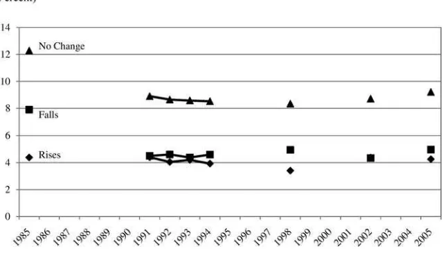
Using the matched SIPP-SSA data, we find that the share of households with large increases in income (Ⳮ50 percent from one year to the next) was about the same as the share of households with large declines in income (ⳮ_{50 percent from one}

year to the next) for most of the sample period (see Figure 1). We find that over 12 percent of households in the matched SIPP-SSA data had a change in total income that exceeded 50 percent between 1984 and 1985; by the early 1990s that share had declined to about 9 percent. It declined further before increasing back to the early 1990s levels by 2005. Decomposing these large changes into large rises and declines separately, we find that, aside from the change between 1984 and 1985, a roughly equal share of households (about 4 percent) experienced a large rise or decline in total household income from one year to the next.

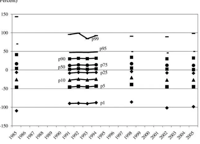
An examination of selected percentiles of the percent change in household income demonstrates substantial dispersion in year-to-year variability. Figure 2 shows the trends in selected percentiles (the 1st, 5th, 10th, 25th, 50th, 75th, 90th, 95th, and 99th) of the distribution of percent changes in total household income from 1985 to 2005. We find that in 2005 the 25th percentile of the arc percent change distribution wasⳮ_{8 percent, the 50th percentile was 1 percent, and the 75th percentile was 12}

(11)

Figure 1

Percentage of Households Whose Income Changed by 50 Percent or More over the Previous Year, Matched SIPP-SSA Data

Source: Various panels of the Survey of Income and Program Participation matched to the administrative earnings data from the Social Security Administration.

Note: Please see the text for a description of the sample. Income is inflated to 2006 dollars using the CPI-U-RS. The year is the second year of a two-year period.

for much of the distribution remain largely unchanged over the 1985 to 2005 period, suggesting that the variability in household income has been relatively constant over the past 20 years. The two exceptions are the patterns in variability at the tails of the distribution: Between 1998 and 2005, the 1st percentile of the percent change distribution became more negative and the 99th percentile grew slightly. This finding seems to agree with those by Sabelhaus and Song (2009) who find that the very bottom of the distribution has significant impacts on their estimates of permanent and transitory shocks of individual earnings.

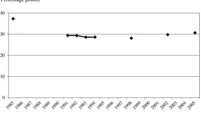
Although most of the distribution of household income volatility was unchanged between 1985 and 2005, the changes in volatility at the 1st percentile and at the 99th percentile result in an initial narrowing and then widening in the dispersion of income volatility over the period. In Figure 3 we show the standard deviation of the arc percent change in household income between 1985 and 2005.13_{The standard} deviation of the year-to-year percent change falls from about 40 percentage points between 1984–85 to 29 percentage points between 1990–91. Over the next few years—during most of the 1990s—the dispersion in the percent change of total household income volatility—is basically unchanged. Beginning with the percent change in incomes between 2001 and 2002, dispersion in household income

(12)

Figure 2

Distribution of the Arc Percent Change in Household Income Over the Previous Year, Matched SIPP-SSA Data

tility rises slightly following the changes at the 1st and 99th percentiles of the percent change distribution shown in Figure 2. In 2005 the standard deviation of the percent change in total household income was 30 percent.

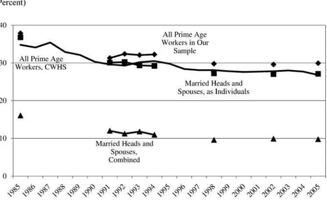
B. Patterns in Individual and Family Earnings Volatility

We step away from total household income volatility for the moment to consider patterns in individual earnings volatility. Differences in estimates of individual earn-ings volatility in the existing literature is often confounded by different definitions of theindividual, be it a prime-age worker (CBO 2007a) or household head (Moffitt and Gottschalk 2008; Dynan, Elmendorf, and Sichel 2008). Here, we compare dif-ferent estimates of individual earnings volatility in the matched SIPP-SSA data (all prime-age workers, heads and spouses as individuals, and heads and spouses com-bined) to estimates of individual earnings volatility from the CWHS. (The CWHS does not contain information linking family members.)

(13)

Figure 3

Standard Deviation of the Arc Percent Change in Household Income Over the Previous Year, Matched SIPP-SSA Data

next declined from about 35 percent in 1985 to nearly 27 percent in 2005 (see Figure 4). Most of the decline occurs during the latter part of the 1980s, after which vol-atility is relatively flat, declines again slightly between 1994 and 1996, and is ba-sically unchanged thereafter. Also plotted in Figure 4 is the same metric for three groups from the matched SIPP-SSA data: all prime-age workers, married heads and their spouses (as denoted in the SIPP), and the combined earnings from married heads and their spouses. All three trends also show a slight decline in individual earnings volatility between the mid-1980s and the early 1990s, but are largely un-changed during the latter half of the 1990s and first half of the 2000s.

(14)

Figure 4

Percentage of Workers Whose Earnings Change by 50 Percent or More Over the Previous Year, Matched SIPP-SSA Data and CWHS

Sources: Various panels of the Survey of Income and Program Participation matched to the administrative earnings data from the Social Security Administration and the Continuous Work History Sample, 1984– 2005.

C. Changes in Household Income Volatility by Household Characteristic

Households with household heads between the ages of 25 and 29 tended to expe-rience higher levels of income volatility, and a greater increase in volatility over the latter part of the sample period, than did those households with older household heads (see Figure 5). Between 1994 and 1998, the share of the youngest households (as measured by the age of the household head) that experienced an income change of 50 percent or more grew from about 9 percent to nearly 12 percent; the share of other households whose incomes changed by 50 percent or more was essentially unchanged over the same period. After 1998, the share of the youngest households that experienced a large income change continued to climb, reaching 13 percent by 2005; changes in household income volatility among older households changed by a much smaller amount, reaching about 9 percent for household heads aged 30–39 and 50–55 and about 8 percent for household heads aged 40 to 49 in 2005.

(15)

Figure 5

Percentage of Households Whose Income Changed by 50 Percent or More Over the Previous Year, Matched SIPP-SSA Data, by Age of Household Head

Sources: Various panels of the Survey of Income and Program Participation matched to the administrative earnings data from the Social Security Administration.

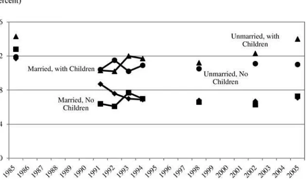
Between married and unmarried households, there are significant differences in the share of households that experience large changes in income over time (see Figure 7). Among married households, the share that saw large changes in income fell between 1985 and 1994 and remained relatively flat thereafter. By the end of the sample period—between 2004 and 2005—about 7 percent of married households (either with or without children) experienced a change in income that exceeded 50 percent. Among unmarried households, a larger share of households had large changes in income: between 2004 and 2005, 11 percent of unmarried households without children and 14 percent of unmarried households with children did so. In addition, while a relatively constant portion of married households saw such large changes, the share of unmarried households with children that had large income changes grew dramatically: by 2005, 14 percent of unmarried households with chil-dren had incomes change by more than 50 percent, up from 11 percent in 1998.

(16)

Figure 6

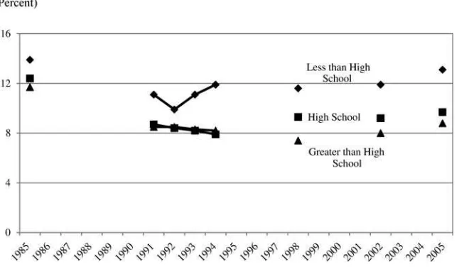
Percentage of Households Whose Income Changed by 50 Percent or More Over the Previous Year, Matched SIPP-SSA Data, by Education of the Head

percent by 2005. This finding is consistent with those patterns found for younger households and households with lower levels of educational attainment.

D. Potential Sources of Income Fluctuations

Knowing the trends in income volatility does not, unfortunately, tell us why income fluctuations occur. To get a better sense of the potential sources of these fluctuations, we examined, descriptively, changes in family structure, sources of income, and hours worked for those whose incomes rose or fell by more than 50 percent relative to those whose incomes did not change as much.

Changes in household structure are associated with changes in income (see Table 3). We find that about 5.5 percent of households with decreases in incomes that exceeded 50 percent had an additional child between 2004 and 2005. While the differences are not statistically significant, about 4 percent of households that ex-perienced a change in income of less than 50 percent had an additional child. House-holds with large decreases in incomes were more likely to get married (3.4 percent) than households that did not have a large change in income (1.8 percent) and this difference is statistically meaningful. Households with large increases in household income were similarly more likely to have gotten married than households with no change in income.

(17)

Figure 7

Percentage of Households Whose Income Changed by 50 Percent or More Over the Previous Year, Matched SIPP-SSA Data, by Household Structure

as likely to have a head enter employment as households with no change in income. In 12 percent of households with large declines in income, the head stopped working altogether. In addition, households with large declines were more than two times more likely to add unemployment insurance as a source of income than households with no change income, but not more likely to add disability as a source of income.

E. Sensitivity of Survey-Based Measures of Income Variability to the Treatment of Imputed Values

In this section, we show how the trends in the survey-based measure of total house-hold income are sensitive to the treatment of imputed values. To do so, we return to the version of the SIPP available to the public; that is, without any administrative earnings information attached to the worker’s record. We then compute our standard measure of volatility—the share of households with large changes in income from one year to the next—for household income based on the survey data with and without imputed values and compare those to estimates of volatility derived from the matched administrative records.

(18)

Figure 8

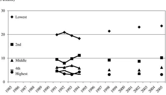
Percentage of Households Whose Income Changed by 50 Percent or More Over the Previous Year, Matched SIPP-SSA Data, by Income Quintile

(19)

Table 3

Percentage of Households Experiencing Changes in Total Household Income due to Changes in Family Structure or Employment

Change in Household Income

the household head marries 3.4** 1.8 3.1*

Employment and income changes

disability is added as an income source

1.2 1.0 1.6

Source: 2004 panel of the Survey of Income and Program Participation matched to the administrative earnings data from the Social Security Administration.

Note: Both the events and the change in real household income are measured between 2004 and 2005. * Statistically different from households with a change in income of less than 50 percent at the 10 percent level; ** at the 5 percent level; *** at the 1 percent level.

V. Discussion

How can we reconcile our results with those in the literature? When we compute trends in income volatility using the publically available SIPP, including observations with imputed earnings, income volatility appears to be increasing in the late 1990s and early 2000s. That increase appears to be data-driven: when we restrict our sample to those households without imputed earnings, household income volatility is roughly flat. Similarly, when we use linked administrative-survey data and replace survey earnings with administrative earnings in constructing household income, our results show no upward trend in volatility.

(20)

Figure 9

The Effect of Imputations on the Percentage with a 50 Percent or Greater Change in the Arc Percent Change in Household Income over the Previous Year

studies agree that both earnings volatility and family income volatility increased between the 1970s and early 1980s.

While we cannot reconcile our results with the divergent set of results from papers using the PSID and other sources of survey data, a comparison with other papers suggests two conclusions. First, there are differences across data sources. The papers that use very similar measures of volatility as we do but use the PSID—Dynan et al. (2008) and Shin and Solon (2009)—tend to find secular trends in earnings and in family income that differ from those found in administrative earnings data and in matched SIPP-SSA data. Second, how one treats the sample affects the trends. In particular, we find that the increasing presence of hot-decked values of income and earnings in the SIPP can lead to an upward bias in the measured trend in year-to-year variability. Imputation alone, however, likely cannot explain the differences; for example, Bollinger et al. (2010)—using the CPS as a panel—find increases in volatility even after eliminating imputed observations.

(21)

Figure 10

The Effect of Imputations on the Standard Deviation of the Arc Percent Change in Household Income over the Previous Year

(22)

VI. Conclusions

This study shows that many workers and households experience rela-tively large changes in their earnings and incomes from one year to the next. Those changes in earnings and income likely have important and far-reaching implications for the households who experience them. Not all of this volatility is necessarily negative nor is it necessarily unanticipated—such changes in earnings or income may be due to changes in family formation, life circumstances, or jobs, to name a few. Fully decomposing volatility into its component reasons is beyond the scope of this paper but is certainly worthy of further research.

We find that a significant number of workers experience substantial changes in their earnings from one year to the next. For example, more than 25 percent of workers saw their earnings change by at least 50 percent between 2004 and 2005. We also find that a significant number of households experience substantial year-to-year variability in their incomes. However, household income tends to vary less than individual worker’s earnings. This is in part because households tend to have more than one source of income: many have multiple earners and may also have other nonlabor income. Moreover, the earnings of other household members and other nonlabor sources of income tend to offset changes in individual worker’s earnings. For example, if one household member were to lose his or her job, another household member might then enter the labor force thereby (at least partially) offsetting the initial loss in household income. As with the trends in earnings volatility, household income volatility declined slightly over the 1985 to 2005 period.

A dynamic labor market is a strength of the U.S. economy. Changes in workers’ incomes from one year to the next are a characteristic of a dynamic labor market: workers move in and out of employment, change jobs (voluntarily or involuntarily), and change locations. At the same time dislocations, job loss, and marital dissolu-tions all can lead to large drops in family incomes that can place a substantial burden on family members. The potential for these burdens has important implications for the design of well-functioning social insurance and tax systems.

References

Allen, R. G. D. 1934. “The Concept of Arc Elasticity of Demand.”Review of Economic Studies1(3):226–29

Autor, David H., Lawrence F. Katz, and Melissa S. Kearney. 2008. “Trends in U.S. Wage Inequality: Re-Assessing the Revisionists.”Review of Economics and Statistics

90(2):300–23

Blank, Rebecca M., and Patricia Ruggles. 1992. “Multiple Program Use in a Dynamic Context: Data from the SIPP.” SIPP Working Paper Series No. 9301, Bureau of the Census, Washington, D.C.

Blundell, Richard, and Luigi Pistaferri. 2003. “Income Volatility and Household

Consumption: The Impact of Food Assistance Programs.”Journal of Human Resources

38 (Supplement): 1032–50.

Bollinger, Christopher R. 1998. “Measurement Error in the CPS: A Nonparametric Look.”

(23)

Bollinger, Christopher R., Bradley Hardy, and James P. Ziliak. 2010. “Earnings and Income Volatility in America: Evidence from Matched CPS. Unpublished.

Bollinger, Christopher R., and Barry T. Hirsch. 2006. “Match Bias from Earnings Imputation in the Current Population Survey: The Case of Imperfect Matching.”Journal of Labor Economics24(3):483–519.

Bound, John, and Alan B. Krueger. 1991. “The Extent of Measurement Error in Longitudinal Earnings Data: Do Two Wrongs Make a Right?”Journal of Labor Economics9(1):1–24.

Bound, John, Charles Brown, Greg J. Duncan, and Willard L. Rodgers. 1994. “Evidence on the Validity of Cross-Sectional and Longitudinal Labor Market Data.”Journal of Labor Economics12(3):345–68.

Cameron, Stephen, and Joseph Tracy. 1998. “Earnings Variability in the United States: An Examination Using Matched-CPS Data.” Unpublished Paper, Federal Reserve Bank of New York.

Congressional Budget Office. 2007a.Trends in Earnings Variability over the Past 20 Years. Washington, D.C.

———. 2007b.Economic Volatility.Testimony of Peter R. Orszag before the Joint Economic Committee, United States Congress, February 28, 2007. Washington, D.C. ———. 2008.Recent Trends in the Variability of Individual Earnings and Household

Income. Washington, D.C.

———. 2009.Changes in the Distribution of Workers’ Annual Earnings Between 1979 and 2007. Washington, D.C.

Cristia, Julian, and Jonathan A. Schwabish. 2009. “Measurement Error in the SIPP: Evidence from Matched Administrative Records.”Journal of Economic and Social Measurement34(1):1–17.

DiNardo, John, Nicole M. Fortin, and Thomas Lemieux. 1996. “Labor Market Institutions and the Distribution of Wages, 1973–1992: A Semiparametric Approach.”Econometrica

64(5):1001–44.

Dooley, Martin D., and Peter Gottschalk. 1984. “Earnings Inequality among Males in the United States: Trends and the Effect of Labor Force Growth.”Journal of Political Economy92(1):59–89.

Dynan, Karen E., Douglas W. Elmendorf, and Daniel E. Sichel. 2008. “The Evolution of Household Income Volatility.”Finance and Economic Discussion Series, Division of Research and Statistics and Monetary Affairs, Federal Reserve Board, 2007–61, Federal Reserve Board, Washington, D.C.

Dynarski, Susan, and John Gruber. 1997. “Can Families Smooth Variable Earnings?”

Brookings Papers on Economic Activity,No. 1: 229–84.

Gosselin, Peter, and Seth Zimmerman. 2007. “Trends in Income Volatility and Risk.” The Urban Institute. Unpublished.

Gottschalk, Peter, and Robert Moffitt. 1994. “The Growth of Earnings Instability in the U.S. Labor Market.”Brookings Papers on Economic Activity1994(2):217–54.

Hacker, Jacob S. 2008.The Great Risk Shift: The New Economic Insecurity and the Decline of the American Dream, Revised and Expanded Edition. Oxford: Oxford University Press. Haider, Steven J. 2001. “Earnings Instability and Earnings Inequality in the United States,

1967–1991.”Journal of Labor Economics19(4):799–836.

Hensher, David A., John M. Rose, and William H. Greene. 2005.Applied Choice Analysis: A Primer.Cambridge University Press: Cambridge.

Hirsch, Barry T., and Edward J. Schumacher. 2004. “Matched Bias in Wage Gap Estimates Due to Earnings Imputation.”Journal of Labor Economics22(3):689–772.

(24)

Jacobs, Elisabeth. 2007. “The Politics of Economic Insecurity.”Issues in Governance Studies, No. 10. The Brookings Institution.

Keys, Ben. 2008. “Trends in Income and Consumption Volatility, 1970–2000.” InIncome Volatility and Food Assistance in the United States, ed. D. Jolliffe and J. P. Ziliak. Kalamazoo, MI: W.E. Upjohn Institute.

Kim, Yong-Seong, Tecla Loup, Joseph Lupton, and Frank Stafford. 2000. “Notes on the ‘Income Plus Files: 1994–1997 Family Income and Components Files.” Unpublished (available at http://psidonline.isr.umich.edu/publications/papers/y_pls_notes.pdf).

Kniesner, Thomas J., and James P. Ziliak. 2002. “Tax Reform and Automatic Stabilization.”

American Economic Review92(3):590–612.

Kopczuk, Wojciech, Emmanuel Saez, and Jae Song. 2010. “Earnings Inequality and Mobility in the United States: Evidence from Social Security Data since 1937”Quarterly Journal of Economics125(1):91–128

Lillard, Lee, James P. Smith, and Finis Welch. 1986. “What Do We Really Know about Wages? The Importance of Nonreporting and Census Imputation.”Journal of Political Economy94(3): 489–506.

Mellow, Wesley, and Hal Sider. 1983. “Accuracy of Response in Labor Market Surveys: Evidence and Implications.”Journal of Labor Economics1(4):331–44.

Moffitt, Robert A., and Peter Gottschalk. 1995. “Trends in the Covariance Structure of Earnings in the U.S.: 1969–1987.” Johns Hopkins University Unpublished Paper. ———. 2002. “Trends in the Transitory Variance of Earnings in the United States.”The

Economic Journal112(March): C68-C73.

———. 2008. “Trends in the Transitory Variance of Male Earnings in the U.S., 1970– 2004.” Boston College Working Paper 697.

Rubin, Donald B. 1987.Multiple Imputation for Nonresponse in Surveys. New York: J. Wiley & Sons.

Sabelhaus, John, and Jae Song. 2009. “Earnings Volatility Across Groups and Time.”

National Tax Journal62:347–64.

Shin, Donggyun, and Gary Solon. 2009. “Trends in Men’s Earnings Volatility: What Does the Panel Study of Income Dynamics Show?” Michigan State University. Unpublished. U.S. Census Bureau. 2001.Survey of Income and Program Participation Users’ Guide

(Supplement to the Technical Documentation) Third Edition, Washington, D.C. ———. 2008.Census SIPP Tutorial. Available at http://www.sipp.census.gov/sipp/tutorial/

SIPP_Tutorial_Beta_version/SIPPtutorialHTML/SIPP_home.htm, accessed January 22, 2008

Welch, Finis. 1979. “Effects of Cohort Size on Earnings: The Baby Boom Babies’ Financial Bust.”Journal of Political Economy87:565–97.

(25)

774

1985 744,697 30,510 47,050 32,440 39,370 37.7 8.3 54.4 1986 769,451 31,720 38,580 32,930 43,460 37.7 8.2 54.0 1987 811,181 31,560 42,270 34,290 70,900 37.8 8.2 53.6 1988 844,084 33,250 69,580 34,030 59,220 37.9 8.2 53.3 1989 872,364 33,170 57,940 34,050 55,050 38.0 8.1 53.1 1990 898,680 33,280 53,860 33,920 52,090 38.1 8.1 52.9 1991 914,545 33,490 51,300 33,340 53,550 38.3 8.1 52.8 1992 923,763 33,100 52,640 34,200 64,110 38.5 8.1 52.7 1993 936,313 33,790 63,060 33,760 58,030 38.7 8.1 52.6 1994 948,055 33,340 57,600 34,120 65,330 38.9 8.1 52.5 1995 970,070 33,350 64,740 34,600 57,150 39.0 8.1 52.3 1996 988,145 33,950 55,770 35,090 64,100 39.2 8.2 52.2 1997 1,002,664 34,520 62,870 36,440 85,970 39.3 8.2 52.0 1998 1,014,531 35,760 84,620 37,780 89,190 39.5 8.2 51.9 1999 1,026,090 37,070 87,830 38,950 113,110 39.7 8.2 51.8 2000 1,038,889 38,250 111,570 39,960 109,730 39.9 8.3 51.7 2001 1,046,428 39,400 101,270 39,440 126,290 40.1 8.3 51.7 2002 1,041,763 39,210 124,700 38,850 95,900 40.2 8.3 51.7 2003 1,032,839 38,620 94,650 38,750 86,720 40.3 8.4 51.6 2004 995,639 38,970 86,850 40,170 117,460 40.8 8.1 51.6 2005 962,037 40,310 118,700 40,790 129,940 41.4 7.8 51.5

Source: Social Security Administration’s Continuous Work History Sample.