The Multi-Scale Interaction between Interest Rate, Exchange Rate and Stock Price

(1)

Munich Personal RePEc Archive

The Multi-Scale Interaction between

Interest Rate, Exchange Rate and Stock

Price

Mohamed Essaied Hamrita and Nidhal Ben Abdallah and

Samir Ben Ammou

Computational Mathematics Laboratory, Faculty of Science,

University of Monastir, Tunisia, Faculty of Economics and

Management Science of Mahdia University of Monastir, Tunisia,

Computational Mathematics Laboratory, Faculty of Science,

University of Monastir, Tunisia

9. October 2009

Online at

http://mpra.ub.uni-muenchen.de/18424/

(2)

The Multi-Scale Interaction between Interest Rate,

Exchange Rate and Stock Price

Mohamed Essaied Hamrita

∗∗∗∗ Computational Mathematics Laboratory

University of Monastir, Tunisia mhamrita@gmail.com

Nidhal Ben Abdallah

Faculty of Economics and Management Science of Mahdia University of Monastir, Tunisia

nidhal.benabdallah@fsegm.rnu.tn

Samir Ben Ammou

Computational Mathematics Laboratory University of Monastir, Tunisia

sam.ben@fsm.rnu.tn

Abstract

This paper examines the multi-scale relationship between the interest rate, exchange rate and stock price using wavelet transform. In particular, we apply the maximum overlap discrete wavelet transform (MODWT) to the interest rate, exchange rate and stock price for US over the period 1990:1- 2008:12 and using the definitions of wavelet variance, wavelet correlation and cross-correlations analyze the association as well as the lead/lag relationship between these series at the different time scales. Our results show that the relationship between interest rate and exchange rate is not significantly different from zero at all scales. On the other hand, the relationship between interest rate returns and stock index returns is significantly different zero only at the highest scales. The exchange rate returns and stock index returns have a relationship bidirectional in this period at longer horizons.

Keywords:

Wavelet analysis, Interest rate, Stock price, Wavelet cross-correlation, Granger

causality.

J.E.L Classification:

C02, C22,

1. Introduction:

The stock markets are becoming an integral part of the economies of many countries. With the introduction of free and open economic policies and advanced technologies, investors are finding easy access to stock markets around the world. The fact that stock

(3)

market indices have become an indication of the health of the economy of a country indicates the importance of stock markets. This increasing importance of the stock market has motivated the formulation of many theories to describe the working of the stock markets.

One piece of information which arrives quite often to the stock markets are interest rates and stock price fluctuations. In theory the interest rates and the stock price have a negative correlation. This is because a rise in the interest rate reduces the present value of future dividends income which should de press stock prices. Conversely, low interest rates result in a lower opportunity cost of borrowing. Lower interest rates stimulate investments and economic activities which would cause prices to rise. On the other hand according to the parity conditions the interest rates and the exchange prices should be related with a negative coefficient. Hence we would expect a relationship between exchange price and stock price with a positive coeffi_cient.

However the empirical studies carried out in the various markets had revealed conflicting results on causality between stock prices and the above economic variables. Mok (1993), verified the causality of daily interest rate, exchange rate and stock prices in Hong Kong for the period 1986 to 1991. The results indicate that the HIBOR (Hong Kong Inter Bank Off_ered

Rate) and the price indices are independent series. As a further extension to the study the relationship between exchange rate and stock price was examined, the research concluded that those series are also independent.

Hashemzadeh and Taylor (1988) have found bi-directional causality present in regression models between money supply and stock returns using stock indexes to estimate market returns. As regards, the interest rate the results are not as conclusive. The direction of causality seems to be mostly running from interest’s rate to stock price but not the other way.

Solnik (1987) found a weak positive relation between real stock return def_{erential and the}

changes in the real exchange rate and he also found that a real growth in the stock market also has a positive influence on the exchange rate.

In this paper, we examine the relationship between interest rate, exchange rate and stock price. We adopt the time series technique based in wavelet analysis. We apply the wavelet cross-correlation between these series based upon the maximum overlap discrete wavelet transform MODWT [Percival, and Mofjeld (1997) and Daubechies (1992)] families of wavelets. The decomposition of a time series on a scale-by-scale basis has the ability to unveil structure at def_{erent time horizons. For example, the wavelet transform produces an}

alternative, known as the wavelet variance, to the periodogram. This variance decomposition may be easily generalized for multivariate time series. Standard time-domain measures of association for multivariate time series (e.g., cross-covariance and cross-correlation) may be defined using the coefficients from the application of the wavelet transform to each series, thus producing the wavelet cross-covariance and wavelet cross-correlation.

The remainder of the paper is organized as follow. The main properties of the wavelets and the analytical def_{erence’s with other filtering methods are dealt with in section 2, where}

(4)

2. Wavelet Analysis:

The series were filtered using wavelet analysis that is a relatively new (at least for economists) statistical tool that, roughly speaking, decomposes a given series in orthogonal components, as in the Fourier approach, but according to scale (time components) instead of frequencies. The comparison with the Fourier analysis is useful first because wavelets use a similar strategy: find some orthogonal objects (wavelets functions instead of sines and cosines) and use them to decompose the series. Second, since the Fourier analysis is a common tool in economics, it may be useful in understanding the methodology and also in the interpretation of results. Saying that, we have to stress the main def_{erence between the two tools. Wavelet}

analysis does not need stationary assumption in order to decompose the series. This is because the Fourier approach decomposes in frequencies space that may be interpreted as events of time-period T (where T is the number of observations). Put diff_{erently, spectral decomposition}

methods perform a global analysis whereas, on the other hand, wavelets methods act locally in time and so do not need stationary cyclical components. Recently, to relax the stationary frequencies assumption a windowing Fourier decomposition that essentially use, for frequencies estimation, a time-period M (the window) event less than the number of observations T. The problem with this approach is the right choice of the window and, more important, its constancy over time. Coming back to wavelets and going into some mathematical detail we may note that there are two basic wavelet functions: the father wavelet

φ and mother wavelets ψ such that:

( ) 1 and (t) 0

R

∫

φ = ψ =

R dt

t (1)

Using wavelets, any function in L2 ( ) can be written as a linear combination of the type

( )

∑∑

_, _, ( )

∑

_, _, ( )

∑∑

_, _, ( ) >

+ =

=

j k k j J k

k j k j k

J k J k

j k

j t S t d t

t

f α φ φ ψ (2)

Where Sj,k = f(t),φj,k(t) anddj,k = f(t),ψj,k(t) are the wavelet coefficients and where , _,

,k jk j ψ

φ the so-called scaling are and wavelet functions, respectively. The formal definition of the father wavelets is the function

( ) 2 /2 (2 )

, t t k

j j

k

j = −

−

− _φ

φ (3)

defined as non-zero over a finite time length support that corresponds to given mother wavelets

( ) 2 /2 (2 )

, t t k

j j

k

j = −

−

− _ψ

ψ (4)

(5)

2.1. The Discrete Wavelet Transform:

Let h1 = (h1,0 , . . . , h1,L-1 ,0, . . . , 0)T denote the wavelet filter coeﬃcients of a Daubechies

compactly supported wavelet for unit scale Daubechies (1992), zero padded to length N by defining h1,l =0 for l > L. A wavelet filter must satisfy the following three basic properties:

0 ; 1

1 0 2 , 1 1 0 ,

1 =

∑

=

∑

− = − = L l l L l l h

h (5)

∑

− = + = 1 0 2 , 1 , 1 0 L l n l lh

h for all non zero integers n. (6)

That is, a wavelet filter must sum to zero (have zero mean), must have unit energy, and must be orthogonal to its even shifts.

Let g1 = (g1,0 , . . . , g1,L-1 ,0, . . . , 0)T be the zero padded scaling filter coefficients, defined via

1 , 1 1 ,

1 ( 1) −−

+ −

= L l

l

l h

g and let X0, . . ., XN-1 be a time series. For scales that N ≥ Lj , where 1 ) 1 )( 1 2 ( − − + = L

L_j j , we can filter the time series using hj to obtain the wavelet coefficients

(

)

1 , 2 2 1 1 2 , ~ 2 1 ) 1 ( 2 , 2 / ,     − ≤ ≤             − − = +

+ j j

t j j j t j N t L W

W (7)

Where,

, 1, . . . , 1 2 1 ~ 1 0 1 , 2 / , =

∑

= − − − = − N L t X h W j j L l t l j j t

j (8)

The Wj,t ~

coefficients are associated with changes on a scale of length τj =2j−1and are

obtained by sub sampling every 2jth of the W~_j_,_tcoefficients, which forms a portion of the maximal overlap discrete wavelet.

However the orthonormal discrete wavelet transform (DWT), even if widely applied to time series analysis in many disciplines, has two main drawbacks: the dyadic length requirement (i.e. a sample size divisible by 2J ), and the fact that the wavelet and scaling coefficients are not shift invariant due to their sensitivity to circular shifts because of the decimation operation. An alternative to DWT is represented by a non-orthogonal variant of DWT: the maximal overlap DWT (MODWT).

2. 2 Maximal Overlap DWT (MODWT):

(6)

∑

− = − − − = − − = = 1 0 mod , 1 , 1 0 mod , 1 , ~ ~ ~ and ~ ~ ~ L l N l t j l t j L l N l t j l t

j g v v hv

w (9)

The wavelet and scaling filters, g~ , _l h~_l are rescaled as _/₂ 2 ~ j j j g

g = , _/₂ 2 ~ j j j h

h = .

Non-decimated wavelet coefficients represent differences between generalized averages of the data on a scale τj =2j−1 (or level j).

MODWT provides the usual functions of the DWT, such as multiresolution decomposition analysis and cross-correlation analysis based on wavelet transform coefficients, but unlike the classical DWT it can handle any sample size; is translation invariant, as a shift in the signal does not change the pattern of wavelet transform coefficients; and provides increased resolution at coarser scales. In addition, MODWT provides a larger sample size in the wavelet correlation analysis and produces a more asymptotically efficient wavelet covariance estimator than the DWT.

2.3 The wavelet variance, covariance, correlation and cross-correlation:

The basic idea of the wavelet variance is to substitute the notion of variability over certain scales for the global measure of variability estimated by sample variance.

The wavelet variance of stochastic process X is estimated using the MODWT coefficients for scale τ_j =2j−1 through:

( )

2 1 1 , 2 _ˆ ˆ 1 ˆ

∑

− − = = N j L k k j j j X W N τ

σ (10)

where Wˆ_j_,_kis the MODWT wavelet coefficient of variable X at scale τ_j . Nˆ_j = N−L_j +1 is

the number of coefficients unaffected by boundary, and L_j =(2j −1)(L−1)+1 is the length

of the scale τj wavelet filter.

Although the wavelet covariance decompose the covariance between two stochastic processes on a scale-by-scale, in some situations it may be beneficial to normalize the wavelet covariance by the variability inherent in the observed wavelet coefficients. The wavelet covariance at scale τ_j can be expressed as follows:

( )

∑

− − = = = 1 1 , , ˆ ˆ ˆ 1 N j L k Y k j X k j j j XY j

XY W W

N Cov τ

τ

γ (11)

Given that covariance does not take into account the variation of univariate time series, it is natural to introduce the concept of wavelet correlation.

The wavelet correlation is simply made up of the wavelet covariance for {Xt, Yt} and wavelet

(7)

( )

( ) ( )

( )

j Y j X

j XY j

XY

Cov

τ σ τ σ

τ τ

ρ ₂ ₂

ˆ ˆ

ˆ = (12)

As with the usual correlation coefficient between two random variables, ρˆ_XY

( )

τ_j ≤1. The

wavelet correlation is analogous to its Fourier equivalent, the complex coherency (Gençay et al (2002, p: 258)).

The wavelet cross-correlation decomposes the cross-correlation between two time series on a scale-by-scale basis thereby making it possible to see how the association between two time series changes as a function of time horizon. Genaçay et al (2002) define the wavelet cross-correlation as:

( )

( ) ( )

( )

j j

j k X j

k

X σ τ σ τ

τ γ τ

ρ

2 1

,

, = (13)

where σ2

( )

τ_j

1 , σ

( )

τj

2

2 are, respectively, the wavelet variances for x1,t and x2,t associated with

scale τj and γX,k

( )

τj the wavelet covariance between x1,t and x2, t – k associated with scale τj. Just as the usual cross-correlation is used to determine lead-lag relationships between two processes, the wavelet cross-correlation should be able to provide a lead-lag relationship on a scale by scale basis (Gençay et al (2002)).

3

Data description and basic statistics:

The analysis was conducted using monthly data for the interest rate of American Treasury securities at 3-month constant maturity provided by the Federal Reserve and the exchange rate between USD and EURO. The closing S&P500 index is used as the indication of the stock price fluctuation. Empirical analysis covers the period form January 1990 to December 2008 providing a 228 observation in total. In this study, we investigate the returns seriesr_t =ln

( ) ( )

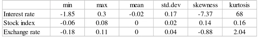
p_t −ln p_t₋₁ . Initially Table1 shows some brief summary statistics for the returns series of interest rate, exchange rate and stock index respectively. From the Table 1, we make the following observations. (a) The mean of returns series is equal zero for all series. (b) Interest rate returns have higher standard deviation than exchange rate and stock index returns showing that the interest rate has higher volatility than the exchange rate and than the stock market. (c) Monthly returns of interest rate tend to have high excess kurtosis.

Both series appear to have similar characteristics, in terms of mean and variation, but a more thorough description is available to use through a multi scale analysis.

min max mean std.dev skewness kurtosis

Interest rate -1.85 0.3 -0.02 0.17 -7.37 68

Stock index -0.06 0.08 0 0.02 0.14 0.16

[image:7.595.67.520.615.680.2]

Exchange rate -0.18 0.11 0 0.04 -0.88 2.04

Table 1 : Descriptive Statistics for returns series

4 Multi Scale Analysis:

(8)

non-zero coefficients Daudechies (1992), with periodic boundary conditions. The application of the translation invariant wavelet transform with a number of scales J = 5 produces five vectors of wavelet filter coefficients, that is w5, w4, w3, w2, w1, and one vector of scaling

coefficients, v5. Since we use monthly data, the wavelet filter coefficients, w5,k, . . . , w1,k, represent progressively finer scale deviations from the smooth behavior, and correspond to 32 – 64, 16 – 32, 8 – 16, 4 – 8 and 2 – 4 months period, respectively.

The main purposes of this paper are to examine the lead-lag relationship and cross-correlation between interest rate, stock market and exchange rate over the various time scales using wavelet analysis. To examine the lead-lag relationship in wavelet analysis, first we test for Granger causality up to level 5. The results of the Granger causality tests are reported in Table 2. As can be seen in Table 2, the stock market and interest rate show a feedback relationship only at higher scales (D4 and D5). The results show also, the unidirectional causality from

stock market to exchange market in various time scales and from interest rate to exchange market at scales D2, D3, D4 and D5.

S5 D1 D2 D3 D4 D5

FX → IR 3.935*

(0.001) 1.850* (0.038) 1.2413 (0.2489) 1.6985 (0.0833) 1.1638 (0.2918) 1.6188 (0.0565)

SM → IR 2.910* (0.002) 1.405 (0.159) 1.2349 (0.2533) 1.6506 (0.0950) 1.9651* (0.0113) 2.8365* (0.0002)

IR → FX 1.225

(0.276) 1.700 (0.063) 2.0217* (0.0183) 2.7712* (0.0032) 3.0075* (0.0001) 1.9646* (0.0126)

SM → FX 2.087*

(0.0271) 2.156* (0.013) 2.8408* (0.0007) 2.3289* (0.0130) 1.4176* (0.1202) 2.4540* (0.0012)

IR → SM 2.1934*

(0.019) 1.399 (0.162) 1.1638 (0.3065) 1.1361 (0.3371) 2.1623* (0.0044) 2.4685* (0.0011)

FX → SM 1.653

[image:8.595.65.527.292.474.2]

(0.0934) 1.480 (0.127) 1.2736 (0.2273) 2.0022* (0.0349) 1.4643 (0.1003) 1.2351 (0.2348) Note – S5 is the original data transformed by the wavelet filter D(4). The significances levels in parentheses. * Significant at the 5% level.

Table 2: Multi scale Granger Causality

Turning to the second purpose of our paper (cross-correlation in various time scale), we examine the cross-correlation between the stock market, interest rate and exchange rate in various time scale.

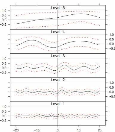
In Figures 1, 2 and 3 we report the estimated wavelet cross-correlations coefficients and the corresponding approximate confidence intervals against time leads and lags for all scales between the interest rate returns and exchange rate returns, interest rate returns and stock index returns and between exchange rate returns and stock index returns respectively. Figure1

shows that, for all scales, the relationship between interest rate and exchange rate in generally not significantly different from zero at all leads and lags (slightly significant at scale 3). This means that interest rate returns and exchange rate returns in this period were independent and historical information of interest rate was not significantly predictive for exchange rate. In

(9)

significant coefficients have positive values. This indicates that the interest rate appreciation (depreciation) was associated with a fall (rise) in stock index. The wavelet cross-correlation provides that exchange rate returns and stock index returns are independent at short horizons (high frequencies). The Figure3 also shows a significant relationship between the two series only at coarsest scale. We note also that significant coefficients have positive values at leads and negative values at lags (scale 5). This means the existence a relationship bidirectional between the two series at long horizons.

(10)

[image:10.595.124.510.72.513.2]

Figure 2: Wavelet cross-correlation between Interest rate and Stock index returns

5 Conclusion:

In this paper we apply a wavelet multi-scaling approach based on a maximum overlap discrete wavelet transform to investigate the relationship between interest rate, exchange rate and stock price over different time scale. Through a scale by scale decomposition of the cross-correlation between two time series we try to shed some light on the scaling properties on the relationship at different time horizons. The main results are summarized as follows:

• The wavelet cross-correlation analysis show that the relationship between interest rate and exchange rate not significantly different from zero at all leads and lags and at all scales.

• The relationship between interest rate and stock index is significantly different zero only at the coarsest scales, i.e. 4–5, which corresponding to longer horizons. The analysis provides evidence about the finding that interest rate returns are leading stock index returns.

(11)

In general it seems that the interest rate and exchange rate series are generally quite independent at the period of studies and at all scales. There was, however a possible unidirectional causality running from interest rate to the stock price but not vice versa at highest scales. Therefore, our results show that a possible bidirectional causality running between exchange rate and stock index only at longer horizons.

Figure 3: Wavelet cross-correlation between Exchange rate and Stock index returns

References:

Daubechies, I. (1992), “Ten Lectures on Wavelets”. Society for Industrial and Applied Mathematics.

Gallegati, Marco (2008), “Wavelet analysis of stock returns and aggregate economic activity” Computational statistics & Data Analysis, 52, 3061– 3074.

(12)

Hashemdah N. and Taylor P. (1988),”Stock prices, money supply and interest rates: The question of causality” Applied economics, 20, 1603-1611.

Harvey A. (1981), “ The Econometric Analysis of Time Series “. Philip Allan.

Kim, S. and F. In (2003), “The relationship between financial variables and real economic activity: Evidence from spectral and wavelet analyses” Studies in Nonlinear Dynamics and Econometrics, 7(4), article 4.

Mok H. M. K. (1993), “Causality of interest rate, exchange rate and stock prices at stock market open and close in Hong Kong” Asia Pacific Journal Of Management, 10, 123-143.

Serroukh, A., Walden, A. T., and Percival, D. B. (2000), “Statistical Properties and Uses of the Wavelet Variance Estimator for the Scale Analysis of Time Series” Journal of the American Statistical Association, 95, 184-196.

Solnik B. (1987), “Using financial prices to test exchange rate models: A note” Journal of Finance 42, 141-149.

Percival, D.B & Walden, Andrew, T (2000), “Wavelet Methods for Time Series Analysis”. Cambridge University Press.

Percival, D. B. and Mofjeld, H. O. (1997), “Analysis of sub tidal coastal sea level fluctuations using wavelets” Journal of the American Statistical Association, 92, 868-880.

Ramsey, J.B., and Lampart, C. (1998a), “The Decomposition of Economic Relationships by Timescale using Wavelets: Expenditure and Income” Study in Nonlinear Dynamics and Economics, 3(1), 23-42.

Ramsey, J.B., and Lampart, C. (1998b), “The Decomposition of Economic Relationships by Timescale using Wavelets: Money and Income” Macroeconomic Dynamics, 2(1), 49-71. Ruey S. Tsay (2005), “Analysis of Financial Time Series” Second edition. Wiley Series in