Staff Site Universitas Negeri Yogyakarta RANCOB DENGAN SAS

(1)

RANCANGAN PERCOBAAN DENGAN SAS

Oleh

Kismiantini, M.Si.

JURUSAN PENDIDIKAN MATEMATIKA

FAKULTAS MATEMATIKA DAN ILMU PENGETAHUAN ALAM

UNIVERSITAS NEGERI YOGYAKARTA

(2)

1

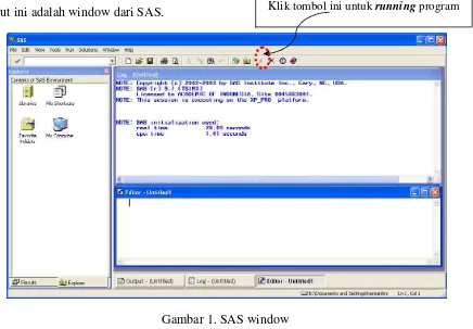
SAS (Statistical Analysis System)

[image:2.595.97.533.112.415.2]

Berikut ini adalah window dari SAS.

Gambar 1. SAS window

1.

Editor

: digunakan untuk memasukkan data dan menganalisis data dengan perintah

tertentu. Untuk memudahkan memasukkan data, ketiklah data pada Microsoft Excell lalu

copy

dan

paste

di Editor SAS.

2.

Log

: menunjukkan bahwa program dapat berjalan dengan sukses atau gagal

3.

Output

: hasil output yang telah di run

(3)

[image:3.595.116.495.56.291.2] [image:3.595.116.497.258.536.2]

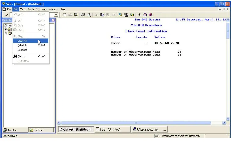
Gambar 2. Output SAS

Gambar 3. Log SAS

(4)

3

RANCANGAN ACAK LENGKAP DENGAN SAS

PROGRAM

data

parasetamol;

input

waktu kadar;

cards

;

7 40

6 40

9 40

4 40

7 40

9 50

7 50

8 50

6 50

9 50

5 60

4 60

8 60

6 60

3 60

3 75

5 75

2 75

3 75

7 75

2 90

3 90

4 90

1 90

4 90

;

proc

glm

data

=parasetamol;

class

kadar;

model

waktu=kadar;

means

kadar/

duncan

;

run

;

LOG

Licensed to ACADEMIC OF INDONESIA, Site 0045663001. NOTE: This session is executing on the XP_PRO platform.

NOTE: SAS initialization used:

real time 28.09 seconds cpu time 1.01 seconds

1 data parasetamol; 2 input waktu kadar; 3 cards;

NOTE: The data set WORK.PARASETAMOL has 25 observations and 2 variables. NOTE: DATA statement used (Total process time):

(5)

29 ;

30 proc glm data=parasetamol; 31 class kadar;

32 model waktu=kadar; 33 means kadar/duncan; 34 run;

OUTPUT

The GLM Procedure Class Level Information

Class Levels Values

kadar 5 40 50 60 75 90

Number of Observations Read 25 Number of Observations Used 25

The GLM Procedure

Dependent Variable: waktu

Sum of

Source DF Squares Mean Square F Value Pr > F Model 4 79.4400000 19.8600000 6.90 0.0012 Error 20 57.6000000 2.8800000

Corrected Total 24 137.0400000

R-Square Coeff Var Root MSE waktu Mean 0.579685 32.14122 1.697056 5.280000

Source DF Type I SS Mean Square F Value Pr > F kadar 4 79.44000000 19.86000000 6.90 0.0012 Source DF Type III SS Mean Square F Value Pr > F

kadar 4 79.44000000 19.86000000 6.90 0.0012

The GLM Procedure

Duncan's Multiple Range Test for waktu

NOTE: This test controls the Type I comparisonwise error rate, not the experimentwise error rate.

Alpha 0.05 Error Degrees of Freedom 20 Error Mean Square 2.88

Number of Means 2 3 4 5 Critical Range 2.239 2.350 2.421 2.470

Means with the same letter are not significantly different.

Duncan Grouping Mean N kadar

A 7.800 5 50 A

B A 6.600 5 40 B

B C 5.200 5 60 C

D C 4.000 5 75 D

(6)

5

RANCANGAN ACAK KELOMPOK LENGKAP DENGAN SAS

PROGRAM

data

rak;

input

bobotbadan kelompok perlakuan$;

cards

;

8

1

A

7

2

A

9

3

A

6

4

A

1

B

0

2

B

3

B

2

4

B

6

1

C

5

2

C

7

3

C

5

4

C

5

1

D

6

2

D

9

3

D

8

4

D

;

proc

glm

data

=rak;

class

kelompok perlakuan;

model

bobotbadan=kelompok perlakuan;

means

perlakuan/

t

;

run

;

LOG

NOTE: PROCEDURE GLM used (Total process time): real time 20.92 seconds cpu time 1.04 seconds

60 data rak;

61 input bobotbadan kelompok perlakuan$; 62 cards;

NOTE: The data set WORK.RAK has 16 observations and 3 variables. NOTE: DATA statement used (Total process time):

79 ;

80 proc glm data=rak; 81 class kelompok perlakuan;

82 model bobotbadan=kelompok perlakuan; 83 means perlakuan/t;

84 run;

NOTE: Means from the MEANS statement are not adjusted for other terms in the model. For adjusted means, use the LSMEANS statement.

OUTPUT

The GLM Procedure Class Level Information

Class Levels Values

kelompok 4 1 2 3 4 perlakuan 4 A B C D

(7)

The GLM Procedure

Dependent Variable: bobotbadan

Sum of

Source DF Squares Mean Square F Value Pr > F

Model 6 103.3750000 17.2291667 18.11 0.0001 Error 9 8.5625000 0.9513889

R-Square Coeff Var Root MSE bobotbadan Mean

0.923506 17.93824 0.975392 5.437500

Source DF Type I SS Mean Square F Value Pr > F

kelompok 3 14.18750000 4.72916667 4.97 0.0265 perlakuan 3 89.18750000 29.72916667 31.25 <.0001

Source DF Type III SS Mean Square F Value Pr > F

kelompok 3 14.18750000 4.72916667 4.97 0.0265

perlakuan 3 89.18750000 29.72916667 31.25 <.0001

The GLM Procedure

t Tests (LSD) for bobotbadan

NOTE: This test controls the Type I comparisonwise error rate, not the experimentwise error rate.

Alpha 0.05 Error Degrees of Freedom 9 Error Mean Square 0.951389 Critical Value of t 2.26216 Least Significant Difference 1.5602

t Grouping Mean N perlakuan

A 7.5000 4 A A

B A 7.0000 4 D B

B 5.7500 4 C

(8)

7

RANCANGAN BUJUR SANGKAR LATIN DENGAN SAS

PROGRAM

data

rbsl1;

input

nilai matakuliah$ perlakuan$ waktu$;

datalines

;

84

Aljabar

A

W1

91

Aljabar

B

W2

59

Aljabar

C

W3

75

Aljabar

D

W4

79

Geometri

B

W1

82

Geometri

C

W2

70

Geometri

D

W3

91

Geometri

A

W4

63

Statistika C

W1

80

Statistika D

W2

77

Statistika A

W3

75

Statistika B

W4

97

Kalkulus

D

W1

93

Kalkulus

A

W2

80

Kalkulus

B

W3

68

Kalkulus

C

W4

;

proc

anova

;

class

matakuliah perlakuan waktu;

model

nilai=waktu matakuliah perlakuan;

means

perlakuan/

tukey

;

run

;

LOG

119 data rbsl1;

120 input nilai matakuliah$ perlakuan$ waktu$; 121 datalines;

NOTE: The data set WORK.RBSL1 has 16 observations and 4 variables. NOTE: DATA statement used (Total process time):

138 ;

139 proc anova;

140 class matakuliah perlakuan waktu; 141 model nilai=waktu matakuliah perlakuan; 142 means perlakuan/tukey;

143 run;

OUTPUT

The ANOVA Procedure

Class Level Information

Class Levels Values

matakuliah 4 Aljabar Geometri Kalkulus Statisti perlakuan 4 A B C D

waktu 4 W1 W2 W3 W4

(9)

The ANOVA Procedure

Dependent Variable: nilai

Sum of

Model 9 1450.500000 161.166667 3.36 0.0768 Error 6 287.500000 47.916667

R-Square Coeff Var Root MSE nilai Mean

0.834580 8.762261 6.922187 79.00000

Source DF Anova SS Mean Square F Value Pr > F

waktu 3 474.5000000 158.1666667 3.30 0.0994 matakuliah 3 252.5000000 84.1666667 1.76 0.2550 perlakuan 3 723.5000000 241.1666667 5.03 0.0446

The ANOVA Procedure

Tukey's Studentized Range (HSD) Test for nilai

NOTE: This test controls the Type I experimentwise error rate, but it generally has a higher Type II error rate than REGWQ.

Alpha 0.05 Error Degrees of Freedom 6 Error Mean Square 47.91667 Critical Value of Studentized Range 4.89559 Minimum Significant Difference 16.944

Tukey Grouping Mean N perlakuan

A 86.250 4 A A

B A 81.250 4 B B A

B A 80.500 4 D B

(10)

9

FAKTORIAL RAL DENGAN SAS

PROGRAM

data

fakral;

input

respons jenis_pupuk varietas_padi;

cards

;

64

1

66

1

70

1

72

1

2

81

1

2

64

1

2

74

1

3

51

1

3

65

1

3

65

2

1

63

2

1

58

2

1

57

2

43

2

52

2

47

2

3

58

2

3

67

2

3

59

3

1

68

3

1

65

3

1

66

3

2

71

3

2

59

3

2

58

3

39

3

42

3

58

4

1

41

4

1

46

4

1

57

4

2

61

4

2

53

4

2

53

4

3

59

4

3

38

4

3

;

proc

glm

data

=fakral;

class

jenis_pupuk varietas_padi;

model

respons=jenis_pupuk varietas_padi jenis_pupuk*varietas_padi;

test

h

=jenis_pupuk

e

=jenis_pupuk*varietas_padi;

run

;

LOG

NOTE: PROCEDURE ANOVA used (Total process time): real time 8:21.67

cpu time 3.00 seconds

144 data fakral;

145 input respons jenis_pupuk varietas_padi; 146 cards;

(11)

NOTE: DATA statement used (Total process time): real time 0.04 seconds

184 ;

185 proc glm data=fakral;

186 class jenis_pupuk varietas_padi;

187 model respons=jenis_pupuk varietas_padi jenis_pupuk*varietas_padi; 188 test h=jenis_pupuk e=jenis_pupuk*varietas_padi;

189 run;

OUTPUT

The GLM Procedure

Class Levels Values

jenis_pupuk 4 1 2 3 4 varietas_padi 3 1 2 3

The GLM Procedure

Dependent Variable: respons

Sum of

Model 11 2277.222222 207.020202 3.31 0.0069 Error 24 1501.333333 62.555556

R-Square Coeff Var Root MSE respons Mean 0.602670 13.49438 7.909207 58.61111

jenis_pupuk 3 1156.555556 385.518519 6.16 0.0029 varietas_padi 2 349.388889 174.694444 2.79 0.0812 jenis_pup*varietas_p 6 771.277778 128.546296 2.05 0.0971

Tests of Hypotheses Using the Type III MS for jenis_pup*varietas_p as an Error Term

(12)

11

PROGRAM

data

fakral;

input

respons lama dosis;

cards

;

96

2

0

98

2

0

94

2

0

90

4

0

94

4

0

92

4

0

92

2

16

88

2

16

90

2

16

88

4

16

92

4

16

94

4 16

92

2

32

94

2

32

84

2

32

78

4

32

82

4

32

74

4

32

74

2

48

74

2

48

68

2

48

0

4

48

0

4

48

0

4

48

50

2

64

50

2

64

54

2

64

0

4

64

0

4

64

0

4

64

;

proc

glm

data

=fakral;

class

lama dosis;

model

respons=lama dosis lama*dosis;

lsmeans

lama*dosis /

pdiff

=all

adjust

=tukey;

run

;

LOG

1124 data fakral;

1125 input respons lama dosis; 1126 cards;

NOTE: The data set WORK.FAKRAL has 30 observations and 3 variables. NOTE: DATA statement used (Total process time):

1157 ;

1158 proc glm data=fakral; 1159 class lama dosis;

1160 model respons=lama dosis lama*dosis;

1161 lsmeans lama*dosis / pdiff=all adjust=tukey; 1162 run;

Dapat diganti dengan

bon

,

(13)

OUTPUT

The GLM Procedure

Class Levels Values

lama 2 2 4

dosis 5 0 16 32 48 64

The GLM Procedure

Sum of

Model 9 37430.53333 4158.94815 503.10 <.0001 Error 20 165.33333 8.26667

R-Square Coeff Var Root MSE respons Mean

0.995602 4.351939 2.875181 66.06667

lama 1 5713.20000 5713.20000 691.11 <.0001 dosis 4 25459.20000 6364.80000 769.94 <.0001 lama*dosis 4 6258.13333 1564.53333 189.26 <.0001

(14)

13

The GLM Procedure Least Squares Means

Adjustment for Multiple Comparisons: Tukey

respons LSMEAN lama dosis LSMEAN Number

2 0 96.0000000 1

2 16 90.0000000 2

2 32 90.0000000 3

2 48 72.0000000 4

2 64 51.3333333 5

4 0 92.0000000 6

4 16 91.3333333 7

4 32 78.0000000 8

4 48 -0.0000000 9

4 64 0.0000000 10

Least Squares Means for effect lama*dosis Pr > |t| for H0: LSMean(i)=LSMean(j) Dependent Variable: respons i/j 1 2 3 4 5 6 7 8 9 10

(15)

FAKTORIAL RAKL DENGAN SAS

PROGRAM

data

fakrakl;

input

y metode intensitas kelompok;

label

y=

'rata-rata nilai tes'

;

cards

;

60 1 1 1

66 1 1 2

77 1 1 3

73 1 2 1

80 1 2 2

82 1 2 3

77 1 3 1

88 1 3 2

86 1 3 3

62 2 1 1

76 2 1 2

62 2 1 3

78 2 2 1

85 2 2 2

91 2 2 3

79 2 3 1

85 2 3 2

88 2 3 3

68 3 1 1

90 3 1 2

83 3 1 3

79 3 2 1

82 3 2 2

87 3 2 3

80 3 3 1

83 3 3 2

89 3 3 3

;

proc

glm

data

=fakrakl;

class

metode intensitas kelompok;

model

y=metode intensitas metode*intensitas kelompok;

lsmeans

metode*intensitas/

pdiff

=all

adjust

=bon;

run

;

LOG

NOTE: PROCEDURE GLM used (Total process time): real time 2:06.45

106 data fakrakl;

107 input y metode intensitas kelompok; 108 label y='rata-rata nilai tes'; 109 cards;

NOTE: The data set WORK.FAKRAKL has 27 observations and 4 variables. NOTE: DATA statement used (Total process time):

137 ;

138 proc glm data=fakrakl;

139 class metode intensitas kelompok;

(16)

15

OUTPUT

The GLM Procedure

Class Levels Values

metode 3 1 2 3 intensitas 3 1 2 3 kelompok 3 1 2 3

Number of Observations Read 27

Number of Observations Used 27

The GLM Procedure Dependent Variable: y rata-rata nilai tes Sum of Source DF Squares Mean Square F Value Pr > F Model 10 1728.222222 172.822222 8.68 <.0001 Error 16 318.444444 19.902778 Corrected Total 26 2046.666667 R-Square Coeff Var Root MSE y Mean 0.844408 5.639224 4.461253 79.11111 Source DF Type I SS Mean Square F Value Pr > F metode 2 156.2222222 78.1111111 3.92 0.0410 intensitas 2 788.6666667 394.3333333 19.81 <.0001 metode*intensitas 4 255.1111111 63.7777778 3.20 0.0412 kelompok 2 528.2222222 264.1111111 13.27 0.0004 Source DF Type III SS Mean Square F Value Pr > F metode 2 156.2222222 78.1111111 3.92 0.0410 intensitas 2 788.6666667 394.3333333 19.81 <.0001 metode*intensitas 4 255.1111111 63.7777778 3.20 0.0412 kelompok 2 528.2222222 264.1111111 13.27 0.0004 The GLM Procedure Least Squares Means Adjustment for Multiple Comparisons: Bonferroni LSMEAN metode intensitas y LSMEAN Number 1 1 67.6666667 1

1 2 78.3333333 2

1 3 83.6666667 3

2 1 66.6666667 4

2 2 84.6666667 5

2 3 84.0000000 6

3 1 80.3333333 7

3 2 82.6666667 8

3 3 84.0000000 9

(17)

Dependent Variable: y

i/j 1 2 3 4 5 6 7 8 9

(18)

17

RANCANGAN SPLIT PLOT DENGAN RAL MENGGUNAKAN SAS

PROGRAM

data

splitplot;

input

i respons tanaman jarak r;

cards

;

1

75.55 1

90

1

2

91.79 2

90

1

3

89.37 3

90

1

4

82.41 1

100

1

5

84.24 2

100

1

6

80.49 3

100

1

7

74.65 1

110

1

8

81.22 2

110

1

9

80.77 3

110

1

10

79.81 1

160

1

11

82.88 2

160

1

12

84.6 3

160

1

13

60.21 1

90

2

14

88.92 2

90

2

15

87.88 3

90

2

16

81.89 1

100

2

17

81.34 2

100

2

18

79.45 3

100

2

19

73.52 1

110

2

20

80.98 2

110

2

21

81.38 3

110

2

22

78.12 1

160

2

23

83.84 2

160

2

24

83.27 3

160

2

25

71.46 1

90

3

26

90.53 2

90

3

27

70.43 3

90

3

28

84.65 1

100

3

29

85.22 2

100

3

30

81.11 3

100

3

31

75.13 1

110

3

32

79.44 2

110

3

33

82.1 3

110

3

34

76.34 1

160

3

35

82.37 2

160

3

36

90.25 3

160

3

;

proc

glm

data

=splitplot;

class

tanaman jarak r;

model

respons=tanaman r(tanaman) jarak tanaman*jarak ;

test

h

=tanaman

e

=r(tanaman);

lsmeans

tanaman*jarak/

pdiff

=all

adjust

=tukey;

run

;

LOG

NOTE: PROCEDURE GLM used (Total process time): real time 4:40.75

280 data splitplot;

(19)

NOTE: The data set WORK.SPLITPLOT has 36 observations and 5 variables. NOTE: DATA statement used (Total process time):

319 ;

320 proc glm data=splitplot; 321 class tanaman jarak r;

322 model respons=tanaman r(tanaman) jarak tanaman*jarak ; 323 test h=tanaman e=r(tanaman);

324 lsmeans tanaman*jarak/pdiff=all adjust=tukey; 325 run;

OUTPUT

The GLM Procedure

Class Levels Values

tanaman 3 1 2 3

jarak 4 90 100 110 160 r 3 1 2 3

The GLM Procedure

Sum of

Model 17 1044.849764 61.461751 3.28 0.0082 Error 18 337.500933 18.750052

R-Square Coeff Var Root MSE respons Mean 0.755850 5.342893 4.330133 81.04472

tanaman 2 451.6972056 225.8486028 12.05 0.0005 r(tanaman) 6 67.2314667 11.2052444 0.60 0.7285 jarak 3 77.2175639 25.7391880 1.37 0.2830 tanaman*jarak 6 448.7035278 74.7839213 3.99 0.0103

Tests of Hypotheses Using the Type III MS for r(tanaman) as an Error Term

tanaman 2 451.6972056 225.8486028 20.16 0.0022

The GLM Procedure Least Squares Means

(20)

19

respons LSMEAN tanaman jarak LSMEAN Number

1 90 69.0733333 1

1 100 82.9833333 2

1 110 74.4333333 3

1 160 78.0900000 4

2 90 90.4133333 5

2 100 83.6000000 6

2 110 80.5466667 7

2 160 83.0300000 8

3 90 82.5600000 9

3 100 80.3500000 10

3 110 81.4166667 11

3 160 86.0400000 12

Least Squares Means for effect tanaman*jarak Pr > |t| for H0: LSMean(i)=LSMean(j) Dependent Variable: respons i/j 1 2 3 4 5 6

1 0.0331 0.9173 0.3707 0.0005 0.0234 2 0.0331 0.4411 0.9525 0.6280 1.0000 3 0.9173 0.4411 0.9943 0.0102 0.3495 4 0.3707 0.9525 0.9943 0.0787 0.9033 5 0.0005 0.6280 0.0102 0.0787 0.7306 6 0.0234 1.0000 0.3495 0.9033 0.7306 7 0.1221 0.9998 0.8336 0.9998 0.2609 0.9987 8 0.0323 1.0000 0.4338 0.9496 0.6360 1.0000 9 0.0419 1.0000 0.5098 0.9740 0.5558 1.0000 10 0.1347 0.9997 0.8586 0.9999 0.2392 0.9978 11 0.0778 1.0000 0.7030 0.9974 0.3736 0.9999 12 0.0058 0.9987 0.1141 0.5394 0.9777 0.9998 Least Squares Means for effect tanaman*jarak Pr > |t| for H0: LSMean(i)=LSMean(j) Dependent Variable: respons i/j 7 8 9 10 11 12

(21)

RANCANGAN STRIP PLOT DENGAN RAK MENGGUNAKAN SAS

PROGRAM

data

stripplot;

input

respons r varietas dosis;

cards

;

2.05 1

1

2.5

1

2

1

2.15 1

3

1

2.6

1

4

1

3.3

1

2

3.25 1

2

3.25 1

3

2

2.95 1

4

2

2.95 1

1

3

2.85 1

2

3

2.75 1

3

1

4

3

2.25 2

1

2.6

2

1

2.5

2

3

1

2.5

2

4

1

3.5

2

1

2

2.95 2

2

3.45 2

3

2

3.05 2

4

2

2.9

2

1

3

2

3

2

3

2.85 2

4

3

2.45 3

1

2.45 3

2

1

2.35 3

3

1

2.25 3

4

1

3.45 3

1

2

3

2

3.5

3

2

3.15 3

4

2

2.95 3

1

3

3.15 3

2

3

2.95 3

4

3

;

proc

glm

data

=stripplot;

class

r varietas dosis;

model

respons=r varietas r(varietas) dosis r(dosis) varietas*dosis

r(varietas*dosis);

test

h

=varietas*dosis

e

=r(varietas*dosis);

run

;

LOG

421 data stripplot;

422 input respons r varietas dosis; 423 cards;

(22)

21

NOTE: DATA statement used (Total process time): real time 0.00 seconds

463 ;

464 proc glm data=stripplot; 465 class r varietas dosis;

466 model respons=r varietas r(varietas) dosis r(dosis) varietas*dosis r(varietas*dosis); 467 test h=varietas*dosis e=r(varietas*dosis);

468 469 run;

OUTPUT

The GLM Procedure

Class Levels Values

r 3 1 2 3 varietas 4 1 2 3 4 dosis 3 1 2 3

The GLM Procedure

Sum of

Model 35 5.39388889 0.15411111 . . Error 0 0.00000000 .

R-Square Coeff Var Root MSE respons Mean 1.000000 . . 2.855556

r 2 0.05597222 0.02798611 . . varietas 3 0.02611111 0.00870370 . . r(varietas) 6 0.13013889 0.02168981 . . dosis 2 4.43930556 2.21965278 . . r(dosis) 4 0.02986111 0.00746528 . . varietas*dosis 6 0.48180556 0.08030093 . . r(varietas*dosis) 12 0.23069444 0.01922454 . .

Tests of Hypotheses Using the Type III MS for r(varietas*dosis) as an Error Term