Full Terms & Conditions of access and use can be found at
http://www.tandfonline.com/action/journalInformation?journalCode=ubes20
Download by: [Universitas Maritim Raja Ali Haji] Date: 12 January 2016, At: 23:52
Journal of Business & Economic Statistics
ISSN: 0735-0015 (Print) 1537-2707 (Online) Journal homepage: http://www.tandfonline.com/loi/ubes20
A New Class of Multivariate Skew Densities,
With Application to Generalized Autoregressive
Conditional Heteroscedasticity Models
Luc Bauwens & Sébastien Laurent
To cite this article: Luc Bauwens & Sébastien Laurent (2005) A New Class of
Multivariate Skew Densities, With Application to Generalized Autoregressive Conditional Heteroscedasticity Models, Journal of Business & Economic Statistics, 23:3, 346-354, DOI: 10.1198/073500104000000523
To link to this article: http://dx.doi.org/10.1198/073500104000000523
Published online: 01 Jan 2012.
Submit your article to this journal
Article views: 211
View related articles
A New Class of Multivariate Skew Densities,
With Application to Generalized Autoregressive
Conditional Heteroscedasticity Models
Luc B
AUWENSCORE and Department of Economics, Université Catholique de Louvain, Louvain-La-Neuve, Belgium (bauwens@core.ucl.ac.be)
Sébastien L
AURENTCREST (CNRS), CORE, Université Catholique de Louvain, Louvain-La-Neuve, Belgium, Department of Quantitative Economics, Maastricht University (laurent@core.ucl.ac.be)
We propose a practical and flexible method to introduce skewness in multivariate symmetric distributions. Applying this procedure to the multivariate Student density leads to a “multivariate skew-Student” density in which each marginal has a specific asymmetry coefficient. Combined with a multivariate generalized autoregressive conditional heteroscedasticity model, this new family of distributions is found to be more useful than its symmetric counterpart for modeling stock returns and especially for forecasting the value-at-risk of portfolios.
KEY WORDS: Multivariate generalized autoregressive conditional heteroscedasticity models; Multi-variate skew density; MultiMulti-variate Student density; Value-at-risk.
1. INTRODUCTION
The increased importance of risk and uncertainty consider-ations in modern economic theory has come with the devel-opment of new econometric time series techniques that allow for the modeling of time-varying means, variances, and cor-relations. The most widespread modeling approach for cap-turing these properties is to specify a dynamic model for the conditional mean and the conditional variance, such as an autoregressive moving average–autoregressive conditional het-eroscedasticity model (ARMA–ARCH) or one of its various ex-tensions (see the seminal work of Engle 1982).
Although there is a huge literature on univariate general-ized ARCH (GARCH) models, much less work is concerned with their multivariate extensions. For this reason, Geweke and Amisano (2001) argued that “while univariate models are a first step, there is an urgent need to move on to multivariate mod-eling of the time-varying distribution of asset returns.” Indeed, financial volatilities move together over time across assets and markets. Recognizing this commonality through a multivariate modeling framework can lead to obvious gains in efficiency and to more relevant financial decision making than can be obtained when working with separate univariate models. (See Bauwens, Laurent, and Rombouts 2003 for a recent survey of multivariate GARCH models.)
The estimation of multivariate GARCH models is commonly done by maximizing a Gaussian likelihood function. Even if this is unrealistic in practice, the normality assumption may be justified by the fact that the Gaussian quasi-maximum likeli-hood (QML) estimator is consistent provided that the condi-tional mean and the condicondi-tional variance are specified correctly. In this respect, Jeantheau (1998) has proved the strong con-sistency of the QML estimator of multivariate GARCH mod-els, extending previous results of Lee and Hansen (1994) and Lumsdaine (1996).
Another well-established stylized fact of financial returns, at least when they are sampled at high frequencies, is that they ex-hibit fat tails (which corresponds to a kurtosis coefficient larger than 3) and are often skewed (see, among others, Alexander 2001; Gourieroux 1997).
As far as financial applications are concerned, and to gain statistical efficiency, it is of primary importance to base model-ing and inference on a more suitable distribution than the multi-variate normal. In particular, Engle and González-Rivera (1991) showed in a univariate framework that the Gaussian QML es-timator of a GARCH model is inefficient, with the degree of inefficiency increasing with the degree of departure from nor-mality, and Peiró (1999) emphasized the relevance of modeling the third and fourth moments in asset pricing models, portfolio selection, and option pricing theories. The challenge to econo-metricians is to design multivariate distributions that are both easy to use for inference and compatible with the skewness and kurtosis properties of financial returns.
The main contribution of this article is to propose a practical and flexible method for introducing skewness in multivariate symmetric distributions. Applying this procedure to the multi-variate Student density leads to a “multimulti-variate skew-Student” density in which each marginal has a specific asymmetry para-meter. We illustrate that, combined with a multivariate GARCH model, this new family of distributions is useful for modeling financial returns and forecasting the value-at-risk (VaR) of port-folios of assets. Indeed, throughout several examples, we find that the multivariate skew-Student density provides better, or at least not worse, out-of-sample VaR forecasts than a symmetric density.
© 2005 American Statistical Association Journal of Business & Economic Statistics July 2005, Vol. 23, No. 3 DOI 10.1198/073500104000000523 346
Bauwens and Laurent: Multivariate Skew Densities 347
The rest of the article is organized as follows. In Section 2 we define the new family of multivariate skew densities. In Sec-tion 3 we investigate the usefulness of the multivariate skew-Student density in a VaR application based on a multivariate GARCH model. In Section 4 we present our conclusions and directions for future research.
2. MULTIVARIATE SKEW DENSITIES
Maximum likelihood (ML) estimation of GARCH models requires an assumption on the distribution of the innovations. To accommodate the leptokurtosis of financial returns, univari-ate GARCH models have been combined with a Student distri-bution by Bollerslev (1987). Indeed, although a GARCH model generates excess kurtosis when combined with a Gaussian conditional density, it does not fully account for the excess kurtosis present in most return series. The Student density has become widely used due to its simplicity and its inherent ability to fit excess kurtosis. It is thus natural to consider its multivari-ate extension as an alternative to the Gaussian when dealing with multivariate GARCH models (see Fiorentini, Sentana, and Calzolari 2003).
As a reminder, the standardized multivariate Student density for the random vectorX∈ ℜkmay be defined as
whereŴ(·)is the gamma function. This density is denoted by
ST(0,Ik, υ). We restrict υ to be larger than 2 to ensure the
existence of the variance matrix (empirically, point estimates smaller than 2 are rarely found).
But the main drawback of this density is that it is symmetric, whereas the distribution of financial returns may be skewed. Consequently, using a more appropriate distribution may lead to improved empirical modeling and financial decision making. Asymmetric densities can be defined by introducing skew-ness in symmetric densities by means of new parameters, such that the symmetric density results as a particular case. In Sec-tion 2.2 we propose a simple and intuitive method for introduc-ing skewness into a multivariate symmetric unimodal density. Before that, we define the notion of symmetry on which we rely.
2.1 Multivariate Symmetry
In the univariate case, symmetry corresponds to g(x)=
g(−x), assuming that g(x) is a unimodal probability density function and that E(X)=0. In the multivariate case, we use the following definition of symmetry of a standardized den-sityg(x).
Definition 1(M-symmetry). The unimodal densityg(x) de-fined onℜk, such that E(X)=0, and var(X)=I
kis symmetric
if and only if for anyx,g(x)=g(Qx)for all diagonal matri-cesQ whose diagonal elements are equal to+1 or to −1. If
Xis a random vector with a density satisfying this definition, then we write
X∼M-sym(0,Ik,g). (2)
In the bivariate case, this definition means that g(x1,x2)=
g(−x1,x2)=g(x1,−x2)=g(−x1,−x2).
Spherically symmetric (SS) densities, defined by the property that the density depends onxthroughx′xonly, that is,
g(x)∝k(x′x), (3) for an appropriate integrable positive function k(·), are M-symmetric. The most well-known examples of SS densities are the standard normal density and the standard Student den-sityST(0,Ik, υ). Johnson (1987, chap. 6) has provided
graphi-cal illustrations of several bivariate SS densities. However, there exist other distributions that have the desired property but are not spherically symmetric. A large class is defined by
g(x)=
(unimodal, with mean 0 and unit variance). One can show that with respect to M-symmetry, (3) and (4) are equivalent if and only if g(·)=N(0,Ik) andgi(·)=N(0,1) ∀i. Nevertheless, if gi(·)=ST(0,1, υ) ∀iandg(·)=ST(0,Ik, υ), then there is a difference between (3) and (4), because the elements of (3) are not mutually independent, whereas those of (4) are. Notice, however, that both multivariate densities have the same univari-ate marginal densities.
2.2 Skew Densities
2.2.1 A Brief Literature Review. Although several mul-tivariate asymmetric densities have been proposed in the literature, we did not find them simple and flexible enough to generate asymmetry and fat tails or to use in ML estimation. Among these, we mention briefly the density of Jones (2001), where the covariances are necessarily positive; Jones (2002); and the heavily parameterized Edgeworth–Sargan density used by Mauleón and Perote (1999) for a bivariate GARCH model. Branco and Dey (2001) proposed a class of skew-elliptical den-sities. They generalized to the complete class of elliptically contoured densities (i.e., densities obtained by linear transfor-mation of a SS density) the multivariate skew-normal density of Azzalini and Dalla Valle (1996).
Asymmetric densities can also be generated using finite mix-tures of symmetric ones. In a GARCH model, Vlaar and Palm (1993) used a mixture of two normal densities. One potential drawback of mixtures is the large number of parameters. Nev-ertheless, this model class coupled with GARCH structures has recently gained attention (see Haas, Mittnik, and Paolella 2002; Alexander and Lazar 2003).
Multivariate stable distributions (see Samorodnitsky and Taqqu 1994) also allow for fat tails and asymmetries with re-spect to the Gaussian density. When this is the case, they are incompatible with finite variance laws. Furthermore, the corre-sponding densities are usually not known in closed form. One must work through the characteristic function, which makes estimation by ML rather difficult.
Fernandez, Osiewalski, and Steel (1995) also proposed a class of continuous multivariate distributions, called
υ-spherical, that are more restrictive in the sense that the skew-ness is the same for every coordinate.
Recently, Ferreira and Steel (2003) introduced a novel class of skewed multivariate distributions and, more generally, a method of building such a class on the basis of univariate skewed distributions. Their method is based on a general linear transformation of a multidimensional random variable with in-dependent components, each with a skewed distribution. They also describe MCMC samplers for conducting Bayesian infer-ence and analyse two applications, one concerning the distrib-ution of various measures of firm size and another on a set of biomedical data.
Finally, a class of multivariate densities that could be of in-terest is the so-called “poly-tdensities,” which contain the mul-tivariate Student density as a particular case. Poly-t densities arise as posterior densities in Bayesian inference (see Drèze 1978), and can be heavily skewed, have fat tails, and even be multimodal. However, the relations between their parameters and moments is complex (see Richard and Tompa 1980 for re-sults on moments of poly-tdensities). Moreover, ML estimation of their parameters, even in the case of iid sampling, is difficult in practice.
2.2.2 A New Class of Multivariate Skew Densities. We generalize to the multivariate case the method proposed by Fernández and Steel (1998) to construct a skew density from a symmetric one. In the univariate case, the idea of the transfor-mation to induce symmetry is to scaleXdifferently for negative and positive values. When X≥0, we multiply it by a positive constant ξ, and when X<0, we divide it by the same con-stant. Assume, without loss of generality, thatξ >1. The effect of this transformation on the symmetric unimodal densityg(x)
centered at 0 is easy to understand; the new density function be-comes more spread over the positive values thang(x), whereas it is less spread over the negative part. The density is skewed to the right. It remains continuous at 0, although its first derivative is not, except in the case of symmetry. The parameterξ clearly determines the direction and the intensity of the skewness.
We can use the same idea for each coordinate of a multi-variate M-symmetric density. LetX∼M-sym(0,Ik,g). Define
krandom variablesWi following independent Bernoulli
distri-butions,
In the univariate case(k=1), this transformation has the effect described earlier; becauseYi= |Xi|ξi is positive ifWi=1 and
It should be clear [see eq. (3) in Fernández and Steel 1998] that ξi2=Pr[Yi≥0|ξi]/Pr[Yi<0|ξi], so that ifξi>1 (<1),
thenh(yi|ξi)is skewed to the right (resp. left). This explains
the parameterization of Pr[Wi=1|ξi]in (5).
In the multivariate case, the transformations defined by (5) and (6) are operated on each of the 2k orthants ofℜk. On
each of these, the densityg(x)is transformed into the density of y conditional ony being in the relevant orthant. Each or-thant corresponds to one and only one realization of the vector
W=(W1,W2, . . . ,Wk)of Bernoulli variables. The conditional
densities on each orthant are then weighted by the probability thatWtakes the corresponding value and added up.
For example, in the bivariate case, definingξ =(ξ1, ξ2)′, we
compute the density ofYas
h(y|ξ)=Pr(W1=1,W2=1|ξ)h(y|W1=1,W2=1,ξ) In the multivariate case, the density is expressed as
h(y|ξ)=2k
This density has the following properties: 1. The mode ofh(y|ξ)is at 0.
2. Each marginal density ofh(y|ξ)can be obtained by trans-forming the corresponding marginal density of g(x) us-ing the relevant part of the transformation defined in (5) and (6). For a univariate marginal, the resulting den-sity is like that in (7), that is, skewed à la Fernández and Steel (1998).
3. ξi2 is a skewness measure determining the skewness of the marginal density ofYi[see the comment after (8) and
sec. 2 in Fernández and Steel 1998]. Right (resp. left) skewness corresponds to logξi>0(<0).
Bauwens and Laurent: Multivariate Skew Densities 349
4. If the cdf ofX is known analytically, then so is the cdf ofY.
5. Following eq. (5) of Fernández and Steel (1998), ifXhas finite moments of orderr, then so doesY. In particular,
E(Yir|ξi)=
ξir+1+(−1)r/ξir+1 ξi+1/ξi 2E(X
r
i|Xi>0). (14)
(See Lambert and Laurent 2001 for the link betweenξi
and the first four moments ofYi.)
6. Finally, if the second-order moments exist, then it is obvi-ous that the elements ofYare uncorrelated (because those ofXare uncorrelated by assumption). Hence ifm is the vector of means andsis the vector of standard deviations of Y, then standardization is achieved straightforwardly by the transformationZ=(Y−m)./s, where “./” de-notes element-by-element division.
2.2.3 Skew-Student Densities. The distribution of finan-cial returns has fat tails and is often skewed. For this reason, it seems natural to apply the skewness filter in (10) to the multi-variate Student density given in (1). Note that as pointed out by a referee, our presentation could be extended to the case where
υ≤2, and most results would hold in this case.
Doing this produces what we call the “standardized skew-Student density,” defined as
not represent additional parameters. This density is denoted by
SKST(0,Ik,ξ, υ), andξis the vector of asymmetry parameters.
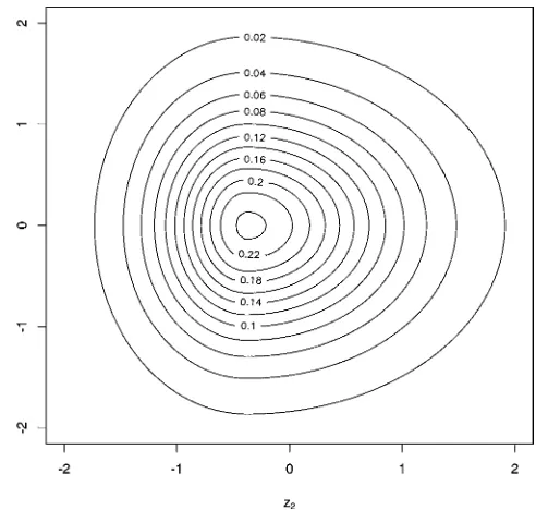
As an illustration, Figure 1 shows the contours of a
SKST(0,I2,ξ,6)density withξ1=1, ξ2=1.3. The contours
show the right-skewness of the density in the direction ofz2
and its symmetry in the direction of z1. We also clearly see
from this “ovoid” that the mode is not at 0, because this is a standardized version.
Obviously, the SKST(0,Ik,ξ, υ) density implies the same
thickness of tails of each marginal density, and its components are not independent. An obvious alternative but close family is obtained by taking the product ofkindependent univariate
Figure 1. Contour of the Bivariate SKST(0,I2, (1, 1.3), 6) Density.
SKST(0,1, ξi, υi)densities. When the degrees of freedom
pa-rameters are all equal (υi =υ ∀i), the marginal densities of
this product are identical to those of the skew-Student density
SKST(0,Ik,ξ, υ), although the joint densities are different. We
thus have a new copula density for asymmetric densities.
3. VALUE–AT–RISK PREDICTION USING A MULTIVARIATE GARCH MODEL
3.1 Data, Models, and Estimates
We use two datasets in the empirical applications. The first dataset consists of three major exchange rates: the Japanese yen (YEN), the Euro (EUR), and the British pound (GBP), all quoted daily against the U.S. dollar, at 12:00 GMT+1 (Source, Reuters). For these series, we have about 12 years of data, from January 1989 to February 2001 (3,066 obser-vations). The EUR/USD series has been obtained from the Deutsche mark (DEM) USD series using the conversion rate 1 EUR/USD=1.95583 DEM/USD.
The second dataset comprises three U.S. stocks of the Dow Jones industrial index (Source, Yahoo Finance) from January 1990 to May 2002 (3,113 daily observations): the Alcoa stock (AA), the Caterpillar Inc. stock (CAT), and the Walt Disney Company stock (DIS). The symbols in parentheses are the short notations (or tickers) for the series, used in the tables and com-ments that follow.
For all price series pit (∀i=1, . . . ,k), daily returns are
defined as yit=100(lnpit −lnpi,t−1). Preliminary univariate
analyses performed on the series allow us to conclude that an AR(p)–GARCH(1,1) model suffices to characterize the dy-namics of the first two conditional moments of the three ex-change rate series, whereas an additional term in the GARCH equation is needed to capture a strong leverage effect for the three stocks. In practice we have used the GJR(1,1)model (see Glosten, Jagannathan, and Runkle 1993) for the stock returns, which adds to the GARCH(1,1)equation the lagged squared
shock when the shock is negative. The order of the autoregres-sive process is set to 1 for AA, EUR, and YEN and to 0 for the other series. Note that the models have been estimated using G@RCH 3.0, an Ox package with a friendly dialog-oriented interface designed for the estimation and forecasting of various univariate ARCH-type models. (See Doornik 2001 for more de-tails about the Ox language and Laurent and Peters 2002 about the G@RCH package.)
Estimation results reveal also that a univariate skew-Student distribution for the innovations (obtained by setting k=1 in Definition 2) improves the quality of the models with respect to the normal and the Student distributions. (Likelihood ratio tests and the Schwarz information criterion clearly favor the skew-Student.) Indeed, the three stocks were found to be positively skewed, whereas the three exchange rates were found to be pos-itively skewed, negatively skewed, and almost symmetric.
Univariate GARCH models are used extensively to compute the VaR of levelα% of a portfolio of assets, over a given time horizon (see Jorion 2000). Indeed, the VaR of levelα% is di-rectly deduced from theαth left or right quantile of the condi-tional distribution of the returns (over the given horizon). The left quantile (such that the probability mass at the left tail is equal to α%) corresponds to the VaR of a long position; the right quantile, to the VaR of a short position. Recall that an in-vestor holds a long position if he has bought an asset, in which case he incurs the risk of a loss of value of the asset, and holds a short position if he has sold an asset and detains cash, in which case he incurs a positive opportunity cost if the asset value in-creases.
Given an estimated parametric GARCH model, one knows the conditional distribution of the return and can compute the needed quantiles. For instance, Giot and Laurent (2003) have shown the supremacy of the univariate skew-Student density over the normal and Student distributions when forecasting the 1-day-ahead VaR of many assets for long and short trading po-sitions (both in-sample and out-of-sample).
Suppose now that one is considering a portfolio of k as-sets. The portfolio return isrt=w′yt, wherew′=(w1, . . . ,wk)
is the vector of shares of the different assets in the portfolio and yt=(y1t, . . . ,ykt)′ is the vector of returns. A univariate
GARCH model can be fit tort and the VaR computed
accord-ingly. However, if the weight vector changes, then the model must be specified and estimated again. In contrast, if a multi-variateGARCH model is fitted, then the multivariate distribu-tion of the returns can be used directly to compute the implied distribution of any portfolio. In other words, there is no need to reestimate the model for a different weight vector. Note that because the distribution assumption is crucial to obtaining ac-curate VaR forecasts in a univariate framework (see Mittnik and Paolella 2000; Giot and Laurent 2003, among others), one can conjecture that this will also be true in the multivariate case, which calls for the use of a flexible density for the innovations. Before presenting the results of the empirical application, we first describe the specification that we choose for the first two conditional moments. Engle (2002) and Tse and Tsui (2002) have proposed extending the constant conditional correlation (CCC) model of Bollerslev (1990) by making the conditional correlation matrix time-varying.
The dynamic conditional correlation (DCC) model of Engle (2002) is defined as
the conditional covariance matrix,σii,tis specified as a
univari-ate GARCH-type equation, andRtis the conditional correlation
matrix.
Thek×ksymmetric positive-definite matrixQtis given by
Qt=(1−α−β)R+αut−1u′t−1+βQt−1, (25)
whereut=(u1t, . . . ,ukt)′,uit=(yit−µit)/√σii,t,Ris thek×k
unconditional covariance matrix ofut, andαandβare positive
scalar parameters satisfying α+β <1. We replace R by its empirical counterpart to make estimation simpler, as suggested by Engle (2002).
Table 1 reports estimation results for the complete samples of the two trivariate models, that is, the series AA–CAT–DIS and EUR–YEN–GBP. Based on the univariate results, we choose univariate AR(p) models (p=0 or 1, according to the series) for the conditional mean equations and a GARCH(1,1) or a GJR(1,1)for the conditional variances (resp. for the exchange rates and the stocks). The models are estimated by ML in one step, assuming a multivariate skew-Student distribution for the innovations(zt). Note that we have conducted a Monte Carlo
study about ML estimates of the parameters of the multivari-ate skew-Student distribution (see Bauwens and Laurent 2002). The results show that even with a sample of 1,000 observa-tions, the ML estimates have a close to normal sampling
dis-Table 1. Estimation Results for Trivariate Models
AA–CAT–DIS EUR–YEN–GBP
NOTE: For each parameter, we report the one-step ML estimate and below it (in parentheses) the corresponding standard error. The estimate of the two-step approach is reported between brackets (third rows).LRT(CCC) andLRT(ST) are LR statistics for the assumption of constant correlations and symmetry with respect to the Student density.
Bauwens and Laurent: Multivariate Skew Densities 351
tribution. This also holds for mean and variance parameters, whether the volatility of the data-generating process is constant or of the GARCH type. Table 1 reports ML estimates using our two trivariate datasets, with corresponding standard errors in parentheses. We report estimates only of the parameters of the DCC part and of the skew-Student distribution.
Table 1 also contains two diagnostic tests for the fitted mod-els. The first test, LRT(CCC), is a likelihood ratio (LR) sta-tistic for testing the restrictionH0:α=β=0, asymptotically ∼χ2(2). In both cases the CCC model is rejected at any con-ventional significance level. This result suggests that the addi-tional flexibility of the DCC model is highly justified. Notice that αˆ + ˆβ is close to unity, so that standard errors must be interpreted with care (although the sample size is large). The second statistic, LRT(ST), is the LR statistic, asymptotically
∼χ2(3), for testing the null hypothesis of symmetry, that is,
H0: logξ1=logξ2=logξ3=0. In both cases, the symmetry
assumption is clearly rejected. In a previous version of this arti-cle (Bauwens and Laurent 2002), we estimated the multivariate GARCH model of Tse and Tsui (2002) with a normal, Student, and skew-Student likelihood on four daily indexes. LR tests and information criteria also clearly favored the latter distribution.
Interestingly, to avoid the dimensionality problem of most multivariate GARCH models, Engle (2002) and Engle and Sheppard (2001) showed that the DCC model can be estimated consistently using a two-step approach. Under the normality as-sumption, the log-likelihood can be decomposed as the sum of a mean-volatility term (that depends only on the parameters of the conditional means and variances) and a second term that depends on the conditional correlation parameters (holding the other parameters fixed). In other words, it is possible to obtain consistent estimates of the DCC model by first estimating k
univariate GARCH-type models and then estimating the con-ditional correlation part, using ut as given. The price to pay
is that the estimates are not fully efficient (because they are limited-information estimators) and that standard errors must be corrected. This issue is not relevant for forecasting the VaR. It could be relevent for estimating the standard error of the fore-cast, although Ruiz and Pascual (2002) showed that this does not seem to matter much.
When using a nonnormal distribution, the decomposition proposed by Engle (2002) is obviously not possible, and one should adopt a one-step approach. However, to stay in the spirit of the DCC model, we also propose to estimate thekunivariate GARCH-type model by QML (to estimateut), and then
esti-mate the correlation part together with the parametersξ andυ
of the skew-Student density.
Estimates are reported between brackets in Table 1 (third rows). Both the one-step and two-step methods give very simi-lar estimates, with a small exception in the case of logξ3in the
exchange rate model.
3.2 Value-at-Risk Forecasts and Evaluations
In a real life situation, GARCH models can be used to deliver out-of-sample forecasts of VaR measures, where the model is estimated on the known returns (up to timetfor example) and the VaR forecast is made for timet+h, wherehis the horizon
of the forecast. In the applications that follow, we use a 1-day horizon.
We denote byµt+1|tandt+1|t the one-step-ahead forecasts
of µt and t, given information up to time t.
Under the normality assumption, the one-step-ahead VaR com-puted at t for long trading positions is given by w′µt+1|t+
of the normal distribution and z1−α the right quantile at α%.
Under the assumption of a multivariate Student distribution, the one-step-ahead VaR is obtained by replacingzα andz1−α
by tα,υ and t1−α,υ, that is, the left and right quantiles of the
Student distribution withυdegrees of freedom.
Under the assumption that zt ∼SKST(0,Ik,ξ, υ), there is
no analytic easy-to-use formula for passing from the condi-tional mean and covariance matrix to the long and short VaR of the portfolio. However, the VaR can be computed using a simple Monte Carlo simulation, as is widely used in VaR com-putations. We just simulate a set of 1-day-ahead returns of the chosen portfolio, as r∗j =w′µt+1|t +zjw′t+1|tw, for j=
1, . . . ,j∗, wherezjis a random draw from theSKST(0,Ik,ξ, υ)
distribution. By definition, the one-step-ahead VaR atα% is de-fined as the empirical quantile at α% of r∗j (over the j∗ sim-ulations. (See Jorion 2000 for a discussion of Monte Carlo techniques in VaR applications.) In the empirical application, we setj∗=100,000.
We use an iterative procedure in which we estimate the DCC model to predict the 1-day-ahead VaR of several portfolios. (We used both the one-step and two-step estimation methods de-scribed earlier, but report only the results concerning the sec-ond approach, because it is much easier to implement and the results hardly differ.) The first estimation sample is the com-plete sample for which the data are available less the last 1,000 observations (about 4 years). We then compare the predicted 1-day-ahead VaR (for both long and short positions) with the observed return, and record both results for later assessment using a statistical test. At theith iteration whereigoes from 2 to 1,000, the estimation sample is augmented to include 1 more day, and the VaRs are forecasted and recorded. Whenever iis a multiple of 50 (about 2 months), the model is reestimated. In other words, we update the model parameters every 50 trading days. We iterate the procedure until all days except the last one have been included in the estimation sample. We then compute corresponding failure rates by comparing the long- and short-forecasted VaR with the observed portfolio return for all days in the 4-year period.
Because the comparison of the VaR forecast and the portfo-lio realization defines a sequence of yes/no observations, it is possible to test H0:f =α against H1:f =α, where f is the
failure rate (estimated byfˆ, the empirical failure rate). Under the null hypothesis, the Kupiec LR statisticLR=2 ln[ ˆfN(1− ˆ
f)J−N] −2 ln[αN(1−α)J−N]is asymptotically distributed as a
χ2(1), whereNis the number of VaR violations,Jis the total number of observations (1,000 in our case), andαis the failure rate of the null hypothesis (see Kupiec 1995). The LR statistic is computed both for long and short trading positions.
Table 2 presents complete VaR results (i.e., p values of the LR statistics) for the following three portfolios composed of
Table 2. VaR Results for AA, CAT, and DIS
w α Normal Student SKST
VaR for long positions
NOTE: Entries arepvalues for the null hypothesisfl=α(i.e., failure rate for the long trading
positions is equal toα, top part of the table) andfs=α(i.e., failure rate for the short trading
positions is equal toα, bottom of the table).wis the weight vector of the portfolio. Grade(5%) summarizes the performance of each model and is defined as the percentage ofpvalues above the 5% critical value (both for long and short trading positions).
the stocks AA, CAT, and DIS:
• 1/3 of AA, 1/3 of CAT, and 1/3 of DIS (equally weighted portfolio)
• 50% of AA, 20% of CAT, and 30% of DIS
• 140% of AA,−20% of CAT, and−20% of DIS.
All models are tested with VaR levels, α, of 5%, 2.5%, and 1%, and their performance is then assessed by computing the failure rate for several portfolios. Estimations have been done using a preliminary version of MG@RCH 1.0, an Ox package dedicated to the estimation and forecast of multivariate GARCH models.
Although the three distributions perform well in predicting the VaR for long positions (top of the table), the empirical evi-dence is very much in favor of the skew-Student density when we consider the short positions (bottom of the table). Indeed, if we use a 5% level for the Kupiec LR statistic, then we re-ject the null hypothesis about the true failure rate in five cases (shown in bold type in the table) for the normal density and in three cases for the Student density, whereas we never reject the skew-Student density. To summarize and compare the results of each model, a performance measure, called Grade(5%), reports the percentage ofpvalues above the 5% critical value (by con-sidering both the long and short trading positions). For instance, because we have 5 rejections for the normal out of 18 cases, its Grade(5%)is 72%, compared with 82% for the Student density and 100% for the skew-Student density.
Next we perform the same exercise on the exchange rate data. We assume that someone is interested in investing in the three currencies (thus we estimate a trivariate model as before), or in pairs (thus we estimate bivariate models). Doing so, we end up with four models and several weight vectors (five for the bivariate cases and three for the trivariate case).
Table 3. Grade(5%) for the Exchange Rates
Series Normal Student SKST
EUR/YEN 90% 97% 97%
EUR/GBP 70% 67% 87%
GBP/YEN 67% 67% 87%
EUR/YEN/GBP 67% 67% 89%
NOTE: In the bivariate cases (first three lines) we consider five weight vectors: (.5, .5), (.2, .8), (.1, .9), (0, 1.0), and (−.1, 1.1). In the trivariate case (last line), the weight vectors are (.1, .8, .1), (−.1, 1.2,−.1), and (.2, .6, .2).
Table 3 presents the performance measure Grade(5%) for various weights. In the bivariate cases (first three lines) we con-sider five weight vectors:(.5, .5),(.2, .8),(.1, .9),(0,1.0), and
(−.1,1.1). In the trivariate case (last line), the weight vectors are(.1, .8, .1),(−.1,1.2,−.1), and(.2, .6, .2).
Broadly speaking, these results are quite similar to those ob-tained for the stocks, because the skew-Student density is never beaten by its symmetric counterparts.
4. CONCLUSION
It is well accepted that high-frequency financial time series are heteroscedastic and leptokurtic, and that volatilities are lated over time across assets and markets. Moreover, asset re-turns may also be skewed, a feature incompatible with the choice of a symmetric density for the innovations of a multi-variate GARCH model.
To improve modeling, we propose a practical and flexible method to introduce skewness in multivariate symmetric dis-tributions. By introducing a vector of skewness parameters, the new class of distributions brings additional flexibility for modeling time series of asset returns with multivariate volatil-ity models. Applying the procedure to the multivariate Student density leads to a “multivariate skew-Student” density, in which each marginal has a different asymmetry coefficient. An easy variant provides a multivariate skew-density that can have dif-ferent tail properties on each coordinate. As a byproduct, a new copula density is obtained.
The usefulness of the multivariate skew-Student density is highlighted throughout a VaR application on several portfolios of assets and currencies. We show that in several cases this den-sity improves the quality of out-of-sample VaR forecasts by comparison with a symmetric one, and that in no case is the performance deteriorated.
The increasing availability of databases providing the intra-day prices of financial assets (e.g., stocks, stock indexes, bonds, currencies) has led to new developments in applied economet-rics and quantitative finance. To reduce the dimension prob-lem inherent to most multivariate volatility models, Andersen, Bollerslev, Diebold, and Labys (2003) proposed computing the daily realized covariance matrix by summing intraday cross-products of returns. Staying in the spirit of the DCC model, they proposed forecasting separately each element of the real-ized covariance matrix (or its Choleski decomposition) using a so-called “ARFIMA” model (see Sowell 1992, among others). This method seems empirically justified, because we have seen in our applications that the DCC was almost integrated, sug-gesting the presence of long-memory and/or structural change in the conditional correlation (see Diebold and Inoue 2001;
Bauwens and Laurent: Multivariate Skew Densities 353
Gourieroux and Jasiak 2001; Granger and Hyung 1999 for discussions about integration vs. long-memory and/or regime switching). Interestingly, Giot and Laurent (2004) have shown, in a univariate framework, how to compute the VaR from the daily realized volatility forecast. Furthermore, they concluded that this method compares very well with the usual daily ap-proach based on a GARCH-type model and that using an appropriate distribution is crucially important in both cases to obtain good VaR forecasts. We conjecture that this result will be transferred to the multivariate case, so that a high-dimensional VaR problem could be solved without imposing strong restric-tions on both the covariance structure and the distribution of the innovations. We leave this topic for future research.
ACKNOWLEDGMENTS
While remaining responsible for any errors in this article, the authors thank the participants of the 2002 Winter Meeting of the Econometric Society in Budapest and of the ESEM meeting in Venice. They are especially grateful to Christian Gouriéroux, Gaëlle Le Fol, Bernard Lejeune, Huston McCulloch, Franz Palm, Jeroen Rombouts, Olivier Scaillet, Jean-Pierre Urbain, the editor, the associate editor, and two referees for helpful comments and suggestions on the initial or revised versions. Sébastien Laurent acknowledges the financial support provided through the European Community’s Human Potential Pro-gramme under contract HPRN–CT-2002-00232, “Microstruc-ture of Financial Markets in Europe.” This article presents research results of the Belgian Program on Interuniversity Poles of Attraction, initiated by the Belgian State, Prime Minister’s Office, Science Policy Programming. The scientific responsi-bility is assumed by the authors.
[Received April 2002. Revised April 2004.]
REFERENCES
Alexander, C. O. (2001),A Practitioners Guide to Financial Data Analysis, New York: Wiley.
Alexander, C. O., and Lazar, E. (2003), “Symmetric Normal Mixture GARCH,” Discussion Papers in Finance 2003-09, ISMA Center.
Andersen, T. G., Bollerslev, T., Diebold, F. X., and Labys, P. (2003), “Modeling and Forecasting Realized Volatility,”Econometrica, 71, 579–626.
Azzalini, A., and Dalla Valle, A. (1996), “The Multivariate Skew-Normal Dis-tribution,”Biometrika, 83, 715–726.
Bauwens, L., and Laurent, S. (2002), “A New Class of Multivariate Skew Den-sities, With Application to GARCH Models,” CORE DP 2002/20. Bauwens, L., Laurent, S., and Rombouts, J. (2003), “Multivariate GARCH
Models: A Survey,” CORE DP 2003/31;Journal of Applied Econometrics, forthcoming.
Bollerslev, T. (1987), “A Conditionally Heteroskedastic Time Series Model for Speculative Prices and Rates of Return,”Review of Economics and Statistics, 69, 542–547.
(1990), “Modeling the Coherence in Short-Run Nominal Exchange Rates: A Multivariate Generalized ARCH Model,”Review of Economics and Statistics, 72, 498–505.
Branco, M. D., and Dey, D. K. (2001), “A Class of Multivariate Skew-Elliptical Distributions,”Journal of Multivariate Analysis, 79, 99–113.
Diebold, F. X., and Inoue, A. (2001), “Long Memory and Regime Switching,”
Journal of Econometrics, 105, 131–159.
Doornik, J. A. (2001),Ox: Object-Oriented Matrix Programming, 3.0, London: Timberlake Consultants Ltd.
Drèze, J. H. (1978), “Bayesian Regression Analysis Using Poly-tDensities,”
Journal of Econometrics, 6, 329–354.
Engle, R. F. (1982), “Autoregressive Conditional Heteroscedasticity With Es-timates of the Variance of United Kingdom Inflation,”Econometrica, 50, 987–1007.
(2002), “Dynamic Conditional Correlation: A Simple Class of Multi-variate Generalized Autoregressive Conditional Heteroskedasticity Models,”
Journal of Business & Economic Statistics, 20, 339–350.
Engle, R. F., and González-Rivera, G. (1991), “Semiparametric ARCH Model,”
Journal of Business & Economic Statistics, 9, 345–360.
Engle, R. F., and Sheppard, K. (2001), “Theorical and Empirical Properties of Dynamic Conditional Correlation Multivariate GARCH,” mimeo, University of California at San Diego.
Fernandez, C., Osiewalski, J., and Steel, M. F. J. (1995), “Modeling and In-ference Withv-Spherical Distributions,”Journal of the American Statistical Association, 90, 1331–1340.
Fernández, C., and Steel, M. F. J. (1998), “On Bayesian Modelling of Fat Tails and Skewness,”Journal of the American Statistical Association, 93, 359–371.
Ferreira, J. T. A. S., and Steel, M. F. J. (2003), “Bayesian Multivariate gression Analysis With a New Class of Skewed Distributions,” Statistics Re-search Report 419, University of Warwick.
Fiorentini, G., Sentana, E., and Calzolari, G. (2003), “Maximum Likelihood Estimation and Inference in Multivariate Conditionally Heteroskedastic Dy-namic Regression Models With StudenttInnovations,”Journal of Business & Economic Statistics, 21, 532–546.
Geweke, J., and Amisano, G. (2001), “Compound Markov Mixture Models With Application in Finance,” mimeo, University of Iowa.
Giot, P., and Laurent, S. (2003), “Value-at-Risk for Long and Short Positions,”
Journal of Applied Econometrics, 18, 641–664.
(2004), “Modelling Daily Value-at-Risk Using Realized Volatility and ARCH-Type Models,”Journal of Empirical Finance, 11, 379–398. Glosten, L. R., Jagannathan, R., and Runkle, D. E. (1993), “On the Relation
Between Expected Value and the Volatility of the Nominal Excess Return on Stocks,”Journal of Finance, 48, 1779–1801.
Gourieroux, C. (1997),ARCH Models and Financial Applications, New York: Springer-Verlag.
Gourieroux, C., and Jasiak, J. (2001), “Memory and Infrequent Breaks,” Eco-nomics Letters, 70, 2941.
Granger, C. W. J., and Hyung, N. (1999), “Occasional Structural Breaks and Long Memory,” Discussion Paper 99-14, University of California at San Diego.
Haas, M., Mittnik, S., and Paolella, M. (2002), “Mixed Normal Conditional Heteroskedasticity,” Working Paper 2002/10, Center for Financial Studies. Jeantheau, T. (1998), “Strong Consistency of Estimators for Multivariate
ARCH Models,”Econometric Theory, 14, 70–86.
Johnson, M. E. (1987),Multivariate Statistical Simulation, New York: Wiley. Jones, M. C. (2001), “Multivariate T and Beta Distributions Associated With
the Multivariate F Distribution,”Metrika, 54, 215–231.
(2002), “Marginal Replacement in Multivariate Densities, With Appli-cation to Skewing Spherically Symmetric Distributions,”Journal of Multi-variate Analysis, 81, 85–99.
Jorion, P. (2000),Value-at-Risk: The New Benchmark for Managing Financial Risk, New York: McGraw-Hill.
Kupiec, P. (1995), “Techniques for Verifying the Accuracy of Risk Measure-ment Models,”Journal of Derivatives, 2, 173–184.
Lambert, P., and Laurent, S. (2001), “Modelling Financial Time Series Using GARCH-Type Models and a Skewed Student Density,” mimeo, Université de Liège.
Laurent, S., and Peters, J.-P. (2002), “G@RCH 2.2: An Ox Package for Estimat-ing and ForecastEstimat-ing Various ARCH Models,”Journal of Economic Surveys, 16, 447–485.
Lee, S. W., and Hansen, B. E. (1994), “Asymptotic Properties of the Maximum Likelihood Estimator and Test of the Stability of Parameters of the GARCH and IGARCH Models,”Econometric Theory, 10, 29–52.
Lumsdaine, R. L. (1996), “Asymptotic Properties of the Quasi Maximum Like-lihood Estimator in GARCH(1,1)and IGARCH(1,1)Models,” Economet-rica, 64, 575–596.
Mauleón, I., and Perote, J. (1999), “Estimation of Multivariate Densities With Financial Data: The Performance of the Multivariate Edgeworth-Sargan Den-sity,” inProceedings of the 12th Australian Finance and Banking Conference, Sidney.
Mittnik, S., and Paolella, M. S. (2000), “Conditional Density and Value-at-Risk Prediction of Asian Currency Exchange Rates,”Journal of Forecasting, 19, 313–333.
Peiró, A. (1999), “Skewness in Financial Returns,”Journal of Banking and Finance, 23, 847–862.
Richard, J.-F., and Tompa, H. (1980), “On the Evaluation of PolytDensity Functions,”Journal of Econometrics, 12, 335–351.
Ruiz, E., and Pascual, L. (2002), “Bootstrapping Financial Time Series,” Jour-nal of Economic Surveys, 16, 271–300.
Samorodnitsky, G., and Taqqu, M. S. (1994),Stable Non-Gaussian Random Processes: Stochastic Models With Infinite Variance, London: Chapman & Hall.
Sowell, F. (1992), “Maximum Likelihood Estimation of Stationary Univariate Fractionally Integrated Time Series Models,”Journal of Econometrics, 53, 165–188.
Tse, Y. K., and Tsui, A. K. C. (2002), “A Multivariate Generalized Autore-gressive Conditional Heteroscedasticity Model With Time-Varying Correla-tions,”Journal of Business & Economic Statistics, 20, 351–362.
Vlaar, P. J. G., and Palm, F. C. (1993), “The Message in Weekly Exchange Rates in the European Monetary System: Mean Reversion, Conditional Het-eroskedasticity and Jumps,”Journal of Business & Economic Statistics, 11, 351–360.