Accumulating foreign exchange reserves, despite their cost and their impacts on other macroeconomics variables, provides some benefits. This paper models such foreign exchange reserves. To measure the adequacy of foreign exchange reserves for import, it uses total reserves-to-import ratio (TRM). The chosen independent variables are gross domestic product growth, exchange rates, opportunity cost, and a dummy variable separating the pre and post 1997 Asian financial crisis. To estimate the risky TRM value, this paper uses conditional Value-at-Risk (VaR), with the help of Glosten-Jagannathan-Runkle (GJR) model to estimate the conditional volatility. The results suggest that all independent variables significantly influence TRM. They also suggest that the short and long run volatilities are evident, with the additional evidence of asymmetric effects of negative and positive past shocks. The VaR, which are calculated assuming both normal and t distributions, provide similar results, namely violations in 2005 and 2008.
© 2013 IRJBS, All rights reserved. Keywords:
Foreign exchange reserve, GJR,
Value-at-Risk, reserves-to-import ratio
Corresponding author: [email protected]
Abdul Hakim
Universitas Islam Indonesia
A R T I C L E I N F O A B S T R A C T
Estimating
Foreign Exchange Reserve Adequacy
INTRODUCTION
The accumulation in foreign exchange reserves (FER) has been widely observed in, especially, developing countries in the last few years. FER is undoubtedly a very important variable in macroeconomics. Rodrik (2006) states that there has been a rapid increase since the early 1990s in foreign reserves held by developing countries. He also states that these reserves have climbed to almost 30 percent of developing countries’ GDP and 8 months of imports.
A country needs to maintain FER for various purposes, such as to finance import, to maintain
exchange rate at a certain range of levels, or to maintain a certain level of exchange rate when the economy applies a fixed exchange rate system (for further discussion, see Monetary and Capital Markets Department, 2013; and Elhiraika and Ndikuma, 2007, among others).
Some strategies have been invented to organize the FER. Antal and Gereben (2011) discuss the strategies to maintain FER before and after the 1997 Asian crises. Moghadam et al. (2011) focus on the precautionary aspect of holding reserves that reflect the key distinguishing characteristics of reserves, namely the availability and liquidity for
potential precautionary reasons. Barnichon (2009) models the optimal level of reserves for low- income countries against external shocks. Borio et al. (2008) focus at trends and challenge to manage foreign exchange reserves.
Besides these benefits, holding FER comes with its price. There are costs need to be born by an economy for holding FER. One of them is the opportunity cost, in terms of the difference between domestic and foreign borrowing rates. Another cost need to be born would be the loss due the value reduction in the denominated foreign exchange reserve. This phenomenon is now faced by China, which has accumulated a huge amount of funds, mostly in US dollar (USD). China suffers loss when USD depreciates. China has now been diversifying the foreign exchange reserve, holding various currencies. The USD proportion in China foreign exchange reserves has declined from 69% to 49% in three years, from 2011-2014 (Ning, 2014). Gosselin and Parent (2005), investigating reserve accumulation by central banks in emerging Asia, suggest that over-accumulation of reserves entails domestic costs such as exchange rate misalignment, loss of monetary control, and sterilization costs. Taking these costs into account would reduce the desired level of international reserves. Yeyati (2006) numerically illustrates the cost of holding reserves that are estimated as sovereign spread on the risk-free return on reserves paid on the debt issued to purchase them. Rodrik (2006) highlights the social cost of foreign exchange reserves. He states that the income loss to most developing countries amounts to close to 1 percent of GDP.
Another aspect of FER is its impact on macroeconomic variables. Fukuda and Kon (2010) find that an increase in foreign exchange reserves raises external debt outstanding and shortens debt maturity. They further suggest that increased foreign exchange reserves may lead to a decline in consumption, but can also enhance investment and economic growth. Chaudry et al. (2011)
investigate the relationships between foreign exchange reserves and inflation by conducting an empirical research on Pakistan since 1960 and find that the rise in FER leads to lower the rate of inflation in Pakistan. Sultan (2011) investigates the aggregate import demand function for India using Johansen’s cointegration method. He finds that there is a long run equilibrium relationship between real imports and real foreign exchange reserves, and that imports are inelastic with respect to foreign exchange reserve.
Considering the benefits, costs, and impacts of holding FER, an economy should organize the FER wisely. There are at least two issues matter, namely, how much FER should be maintained, and the currencies composition of the FER. Regarding the first issue, Zeng (2012) investigates whether the Chinese foreign exchange reserves have been too large. He finds that the Chinese actual foreign exchange reserves greatly exceeded the 3-month import foreign exchange demands and also that the optimal foreign exchange reserves demands were calculated to be 40% of the total foreign debt balance. Antal and Gereben (2011) find that international reserves are likely to increase further, which might generate further tensions in the global financial system. To avoid global imbalances, international coordination and alternative sources of foreign exchange liquidity should be reinforced. Siregar and Rajan (2003) investigate ways to generate the liquidity yield from holding reserves. They suggest that pooling of reserves with other East Asian economies may be a means by which Indonesia and other regional economies are able to generate such extra resources.
high, VaR increases.
To organize FER, the first step is to construct a model on it. Various attempts have been made on this matter. Various regression techniques have been applied such as multiple regression (Romero, 2005; Sianturi, 2011; and Alam and Rahim, 2013, among others), Granger causality test (Akdogan, 2010), and dynamic model averaging (DMA), dynamic model selection (DMS) random walk, recursive OLS-AR, recursive OLS with all predictive variables models, or Bayesian model averaging (BMA) (Gupta et al., 2014).
Various independent variables have also been used to explain FER such as export and import (Akdoban 2010 and Sianturi, 2011), current account balance (Wijnholds and Kapteyn, 2001; Gupta and Agarwal, 2004; Romero, 2005; and Alam and Rahim, 2013), capital and financial account balance (Wijnholds and Kapteyn, 2001; Gupta and Agarwal, 2004; and Alam and Rahim, 2013), exchange rates (Wijnholds and Kapteyn, 2001; Gupta and Agarwal, 2004; Romero, 2005; and Alam and Rahim, 2013), interest rate differential or opportunity cost (Wijnholds and Kapteyn, 2001; Gupta and Agarwal, 2004; and Akdoban, 2010; and Gupta et al. 2013), economic size or GDP (Wijnholds and Kapteyn, 2001 and Gupta and Agarwal, 2004), possibility of capital flight (Wijnholds and Kapteyn, 2001 and Gupta and Agarwal, 2004), and average propensity to import, Romero (2005), and consumption differentials (Akdoban, 2010).
Most of these researches are able to explain the behaviour of FER. However, these models do not answer the question of how much foreign exchange reserves should be maintained. The IMF, through its Monetary and Capital Markets Department (2013) have made guidelines in 2001, which then revised in 2012, for foreign exchange reserve management. They meant for helping strengthen the international financial architecture, to promote policies and practices that contribute
to stability and transparency in the financial sector, and to reduce external vulnerabilities of member countries. The objectives of the guidelines are to ensure, among others, adequate foreign exchange reserves are available for meeting a defined range of objectives. However, they do not specifically mention the need to save the import of goods and services from other countries.
According to rule of thumb, the position of foreign currency in a country is said to be safe if the FER is enough to finance the country’s import for at least three months (see Gupta et al., 2013 and Zheng, 2013; among others). If, to make it simple, each year we import an amount of USD 12, throughout the year we have to be ready with, at least, ¼ times USD 12 = 3 USD. The ratio, ¼, comes from 3 months divided by 12 months. In another word, the FER-to-import ratio should be at least 0.25. As an alternative, this paper proposes to find the risky ratio level assuming that the ratio follows a certain type of distribution. Assuming this distribution, the risky ratio can be calculated as the Value-at-Risk (VaR). The VaR is calculated as the mean of the distribution minus the product of statistical value (say 1.65 for 95% assuming normal distribution, one side estimate) and the standard deviation of the distribution. In this case, we assume that in common situation, foreign exchange reserves are always enough to support imports. In such a case, the ratio will be higher than the VaR. The ratio will be lower than the VaR only in non-common situation, namely when there are unexpected shocks. Such shocks might come from domestic or foreign sources. Therefore, during a crisis, we can expect that the ratio will be lower than the corresponding VaR.
variable in daily basis. For discussion about VaR, please read Brooks et al. (2005), Bhattacharyya et al. (2008), and Bao et al. (2006), among others. For conditional VaR, please read Chan et al. (2007), Jabr (2005), and Ku and Wang (2008), among others.
The standard deviation used in this paper is a conditional standard distribution assuming that the variance of the model is volatile. We can use the help of GARCH family models to model such volatility. Therefore, this paper uses conditional VaR to model and estimate such foreign exchange reserves. For the usefulness of GARCH family model in modelling volatility, volatility spillovers, and conditional correlations, please refer to McAleer (2005) and McAleer et al. (2007).
METHODS
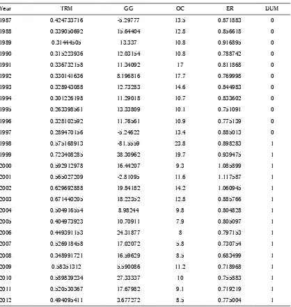
From the above discussion, this paper models TRM uses some variables that influence total foreign reserve, namely gross domestic product, exchange rates, and opportunity cost. To avoid regressing non-stationary variables, this paper uses GDP growth (GG) instead of GDP. GDP is included in the model to represent the economic size, in which reserves are expected to rise with population and real per capita
The exchange rate uses in this paper is USD/ IDR. This variable is included in the model because it influences the need of the reserves to be accumulated. The higher the exchange rate flexibility, the smaller the reserves that needs to be accumulated.
As of the saying, there is no such thing as free lunch, accumulating reserves also has its cost. The opportunity cost is included in the model to measure the cost of accumulating the reserves. This paper uses the difference between Indonesian lending rate and US lending rate.
The dependent variable in this paper is the ratio between total foreign reserve (TRM), assuming
that one of the main goal in accumulating foreign reserves is to provide enough funds to import.
As discussed, this paper models the TRM using both conditional mean and conditional variance. The conditional variance is then employed to calculate the VaR. Different from non-conditional VaR, where the value is calculated as the mean plus or minus the distribution value times the standard deviation, this paper uses conditional VaR since the standard deviation (volatility) is a conditional volatility, modeled by a family of GARCH model. This paper uses GJR model by Glosten et al. (1993), a family of univariate GARCH model which, in addition to traditional GARCH model, also accommodates the possibility of asymmetric impact of negative and positive shocks on the conditional variance. The model can be written as follows:
(1)
(2)
(3)
where . If r = s =1, , , , and are sufficient condition to ensure that the conditional variance
h
t≥
0
. Theshort-persistence of positive (negative) shocks are given by a1(a1 + g1) . When the conditional shocks,
h
t, follow a symmetric distribution, the expected short-run persistence is a1+ g1/2, and the contribution of shocks to expected long-run persistence is a1 + g1/2 + b1 (see McAleer (2005)).All data are taken from The World Bank (2014), except for the ER, which is from fxtop.com, available at http://fxtop.com/en/historical-exchange-. TRM is calculated as the ratio of Total Foreign Exchange Reserve divided by Import. GG is the growth of
GDP, calculated by the formula of GGt = 1n(GDPt /
of accumulating total reserve, calculated as the difference between Indonesian lending rate and the US lending rate. ER is the exchange rate, which is IDR/USD in this case. DUM is a dummy variable which takes zero for years prior the crises (1987 – 1997) and one for years post the crises (1998-2012).
RESULTS AND DISCUSSION
To make sure that the estimation is not spurious, this paper tests the variables included in the model. Using a Dickey-Fuller test, the results are presented in Table 2. It can be inferred that the statistical values (in absolute values) are bigger
than that of the critical values (in absolute values) in 5% significance level. Therefore, it can be concluded that all variables are stationary at that level.
Variables t-stat 5% t-critical
GG -5.181613 -1.955020
OC -3.372349 -1.955681
ER -2.019590 -1.955681
TRM -2.073725 -1.955020
Table 2. DF Test for Unit Root
Year TRM GG OC ER DUM
1987 0.424733716 -5.29777 13.5 0.871883 0
1988 0.339050692 15.64404 12.8 0.856618 0
1989 0.31444505 13.337 10.8 0.916895 0
1990 0.315223936 12.03154 10.8 0.788742 0
1991 0.336732158 11.34092 17 0.811868 0
1992 0.330141636 8.196816 17.7 0.769998 0
1993 0.328943088 12.73283 14.6 0.844983 0
1994 0.301226198 11.29018 10.7 0.833602 0
1995 0.263398561 13.33809 10.1 0.751091 0
1996 0.328102592 11.76561 10.9 0.775139 0
1997 0.289470156 -5.24622 13.4 0.885013 0
1998 0.575168913 -81.5559 23.8 0.898283 1
1999 0.723408285 38.30962 19.7 0.939475 1
2000 0.592912978 16.44207 9.3 1.085899 1
2001 0.565027209 -2.81095 11.6 1.117587 1
2002 0.629692888 19.84182 14.2 1.060945 1
2003 0.671440205 18.22352 12.8 0.885766 1
2004 0.504916554 8.98244 9.8 0.804828 1
2005 0.404973923 10.70911 7.9 0.805097 1
2006 0.449391153 24.31877 8 0.797153 1
2007 0.526918458 17.02072 5.8 0.730754 1
2008 0.348991721 16.59629 8.5 0.683499 1
2009 0.58351312 5.590086 11.2 0.718968 1
2010 0.589839234 27.33337 10 0.755883 1
2011 0.520530367 17.67982 9.1 0.719219 1
2012 0.494095411 3.677272 8.5 0.775004 1
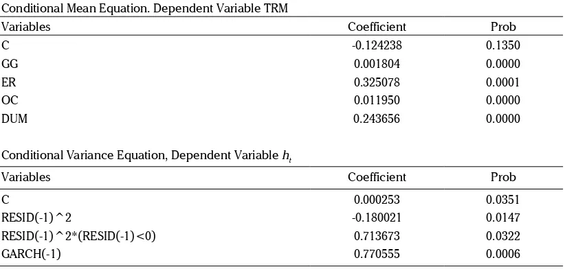
The estimation results of the model are presented in Table 3. It can be inferred that all variables in conditional mean equations are significant even at 1% level. All the independent variables influence TRM in positive fashions.
It can be learned that the higher the GDP growth, the higher the TRM, reflecting the need of more foreign reserves, assuming that import is constant. It can be learned as well that the higher the exchange rates, the higher the TRM. This means that as Indonesian Rupiah is weaken against the USD dollar, the economy needs to accumulate more reserves, since perhaps more imports is expected. In addition, the higher the OC, the higher the foreign reserves. Last but not least, the dummy variable also suggests the positive impact on the TRM. This means that post the 1997 crises, the TRM increases. It is commonly understood that when a country moves from a fixed exchange rate rezim to a floating one, it will accumulate less foreign reserves. This is so because the country does not need to maintain a certain level of exchange rates. The fact that Indonesia has higher TRM following the crises perhaps suggesting that the impact of the aforementioned three independent variables are so strong that the impact surpasses that impact of the crises.
The results of the conditional variance equation suggest that the ARCH and GARCH impacts on the conditional variance are significant. This means that the variance is volatile in both the short and long runs. In addition, the results also suggest that the asymmetry of the negative and positive impacts is evident. This means that the negative shock has stronger impact than that of the positive one.
To estimate the VaR, the following formula is applied
1
)
(
−
−=
t t tt
E
Y
X
z
h
VaR
(4)where VaRt is Value-at-Risk at time t, and Xt
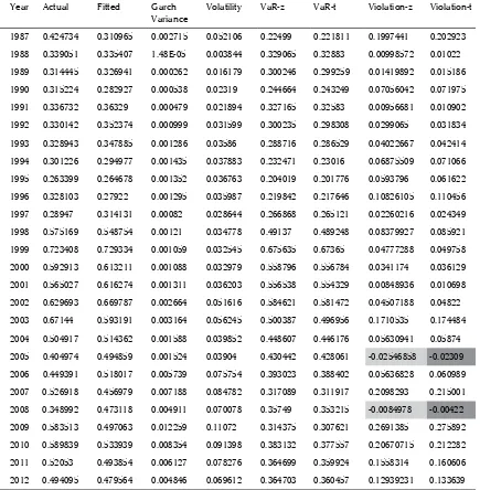
represents all independent variables in the model. The z value is the standardized normal distribution value calculated using a certain confidence level. This z value can be replaced with t value if it is assumed that t-student distribution is considered as the more appropriate distribution. The result is in Table 4.
Table 4 lists the actual, fitted, and GARCH variance values. Taking the square root of the GARCH variance value, we get the conditional standar deviation, or the conditional volatility, which is
Conditional Mean Equation. Dependent Variable TRM
Variables Coefficient Prob
C -0.124238 0.1350
GG 0.001804 0.0000
ER 0.325078 0.0001
OC 0.011950 0.0000
DUM 0.243656 0.0000
Conditional Variance Equation, Dependent Variable ht
Variables Coefficient Prob
C 0.000253 0.0351
RESID(-1)^2 -0.180021 0.0147
RESID(-1)^2*(RESID(-1)<0) 0.713673 0.0322
GARCH(-1) 0.770555 0.0006
nothing but the value of
h
t . Applying the VaRformula in (4), we can get the value of VaR, both assuming normal and t distribution (column 6 and 7).
Comparing the actual TRM and the corresponding VaR-z, we can find two violations, namely years where TRM is lower than VaR-z, which are in 2005 and 2008. This means that in 2005 and 2008, the TRM are so low, lower than the safe level, namely the VaR level. A comparison between actual TRM and VaR-t provides exactly the same result with previous comparison.
The violation in 2005 might due to the hurricanes Katrina, which hit the Gulf Coast of the USA, one of the biggest natural disasters in US history, and Hurricane Rita that occurred soon after the Katrina. They created loss of more than USD 200 billion, 400,00 loss of jobs, 275,000 destroyed homes. This perhaps influences the trade vis-à-vis Indonesia. The violation in 2008 might due to the crash in the 2008 US capital market. Even though there is no violation in 1997, but actually the actual TRM (0.2897) is very close to the corresponding VaR-z (0.266868) and corresponding VaR-t (0.265121).
Year Actual Fitted Garch
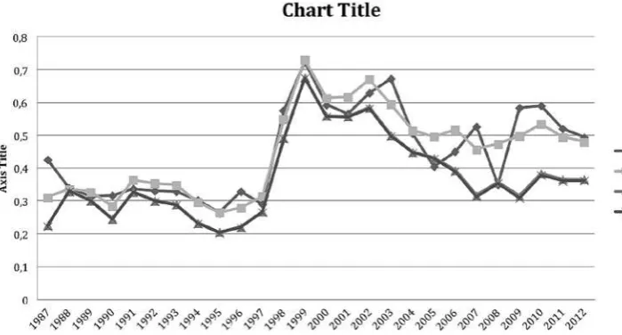
The comparison between the actual TRM, the fitted value, VaR-z, and VaR-t is depicted in Figure 1. To analyze the violation of TRM with respect to VaR-z, both graphs are presented in Table 2. We can see two violations, both in year 2005 an 2008. To analyze the violation of TRM with respect to VaR-t, both graphs are presented in Table 3. Similar with the aforementioned violation, we can also see two violations in this comparison, namely both in year 2005 an 2008.
MANAGERIAL IMPLICATIONS
This paper models the Value-at-Risk of total foreign exchange reserves to import ratio. When the ratio
is lower than the Value-at-Risk, this means that foreign exchange reserve is not enough to support imports in such a way that it might endanger the whole economic system of the country. Therefore, the model can be used as a precautionary warning about such situation.
The model can be developed to accommodate forecast of the VaR of such ratio in the future. The forecast can be developed by considering the va-lues of independent variables of interest, namely GG (growth of GDP), OC (opportunity cost of accu-mulating total reserve, calculated as the difference between Indonesian lending rate and the US
len-Figure 1. Comparing Actual, Fitte, VaR-z, and VaR-t Values
ding rate), and ER (exchange rate, which is IDR/ USD). With such forecast, for the nearest two or three months, the government will have sufficient time to prepare policies to avoid such unfortunate situation.
The calculation of conditional Value-at-Risk em-ploying conditional volatility which are modeled using a GARCH family model allow the estimation of annual Value-at-Risk. If monthly data is readily available, monthly conditional Value-at-Risk will be easily calculated, which makes it possible to estimate monthly risk of the availability of foreign exchange reserves.
CONCLUSION
This paper models the behavior of total foreign exchange reserves to import ratio, a very important variable in an economy. To estimate the critical
value in which the ratio is not adequate to support import, this paper uses Value-at-Risk (VaR), a measure famous in finance. Different from conventional VaR, this paper uses conditional VaR, namely VaR based on conditional volatility, which is provided by the GJR model, a family of GARCH model.
The model gives strong significant result, both in the conditional mean model (first moment) and conditional variance model (second moment). The VaR built on both normal (z) and t distributions provide similar results, namely both conditional VaR are lower than the actual TRM. This means that most of the time, the positions of total foreign reserves in Indonesia is safe. However, there two violations occurred, namely in 2005 and 2008. The results are supported by both normal and t distributions.
Acknowledgement
The author acknowledges the funding provided by Direktorat Jenderal Tinggi, Departemen Pendidikan Nasional, Republik of Indonesia, under the scheme of Hibah Kompetensi, 2013.
R E F E R E N C E S
Akdogan, K. (2010). Foreign Exchange Reserve Demand: An Information Value Approach. Central Bank Review, Central Bank of the Republic of Turkey, Vol. 10 (July 2010), 33-44.
Alam, M. Z. and Rahim, M. A. (2013). Foreign Exchange Reserves: Bangladesh Perspective. International Journal of Finance & Banking Studies, 12(4), 1-12.
Antal, J. and Gereben, A. (2011). Foreign Reserve Strategies for Emerging Economies - Before and After the Crisis. Magyar Nemzeti Bank (MNB) Bulletin, April, 7-19.
Bao, Y., Lee, T. H. and Saltoglu, B. (2006). Evaluating Predictive Performance of Value-at-Risk Models in Emerging Markts: A Reality Check. Journal of Forecasting, 25, 101-128.
Barnichon, R. (2009). The Optimal Level of Reserves for Low Income Countries: Self Insurance against External Shocks. IMF Staff Papers, Vol.56(4), 852-875.
Bhattacharyya, M., Chaudhary, A. and Yadav, G. (2007). Conditional VaR Estimation using Pearson’s Type IV Distribution. European Journal of Operational Research, 191, 386-397.
Borio, C., Galati, G. and Heath, A. (2008). FX Reserve Management: Trends and hallenges. BIS Papers, No 40.
Brooks, C., Clare, A. D., Molle, J. W. D., and Persand, G. (2005). A Comparions of Extreme Value Theory Approaches for Determining Valut at Risk. Journal of Empirical Finance, 12, 339-352.
Chan, N. H., Deng, S. J., Peng, L., and Xia, Z. (2007). Interval Estimation of Value-at-Risk based on GARCH Models with Heavy-tailed Innovations. Journal of Econometrics, 137, 556-576.
Chaudry, I. S., Akhtar, M. H., Mahmood, K. and Faridi, M. Z. (2011). Foreign Exchange Reserves and Inflation in Pakistan: Evidence from ARDL Modelling Approach. International Journal of Economics and Finance, 3(1), 69-76.
International Research Journal of Finance and Economics, 21, 76-92.
Elhiraika, A. and Ndikumana, L. (2012). Reserves Accumulation in African Countries: Sources, Motivations, and Effects. Working Paper No. 2007-12, Department of Economics, University of Massachusetts Amherst.
Fukuda, S. and Kon, Y. (2010). Macroeconomic Impacts of Foreign Exchange Reserve Accumulation: Theory and International Evidence. ADBI Working Paper 197. Tokyo: Asian Development Bank Institute.
Glosten, L. R., Jagannathan, R. and Runkle, D. (1993). On the Relation between the Expected Value and the Volatility of the Normal Excess Return on Stocks. Journal of Finance, 48, 1779– 1801.
Gosselin, M-A. and Parent, N. (2005). An Empirical analysis of Foreign Exchange Reserves in Emerging Asia. Bank of Canada Working Paper 2005-38.
Gupta, A. and Agarwal, R. (2004). How Should Emerging Economies Manage their Foreign Exchange Reserves?” Retrieved from SSRN: http://ssrn.com/abstract=466783 or http://dx.doi.org/10.2139/ssrn.466783
Gupta, R., Hammoudeh, S. Kim, W. J., and Simo-Kengne, B.D. (2013). Forecasting China’s Foreign Exchange Reserves Using Dynamic Model Averaging: The Role of Macroeconomic Fundamentals, Financial Stress and Economic Uncertainty. Department of Economics Working Paper Series N0. 2013-38, University of Pretoria.
Jabr, R. A. (2005). Robust Self-Scheduling under Price Uncertainty Using Conditional Value-at-Risk. IEEE Transactions on Power Systems, 20(4), 1852-1858.
Ku, Y. H. H. and Wang, J. J. (2008). Estimating Portfolio Value-at-Risk via Dynamic Conditional Correlation MGARCH Model – An Empirical Study on Foreign Exchange Rates. Applied Economics Letters, 15, 533-538.
Mcaleer, M. (2005). Automated Inference and Learning in Modeling Financial Volatility. Econometric Theory, 21, 232–261. Mcaleer, M., Chan, f. and Marinova, D. (2007). Econometric Analysis of Asymmetric Volatility: Theory and Application to
Patents. Journal of Econometric, 139, 259–284.
Moghadam, R., Ostry, J. D. and Sheely, R. (2011). Assessing Reserve Adequacy. International Monetary Funds Paper, available at http://www.imf.org/external/np/pp/eng/2011/021411b.pdf.
Monetary and Capital Markets Department (2013). Revised Guidelines for Foreign Exchange Reserve Management. International Monetary Funds.
Ning, Z. (2014). Testing Time for China;s Foreign Exchange. China Daily, 2014, 02, 18, 1:16. Retrieved from http://usa.chinadaily. com.cn/business/2014-02/18/content_17289655.htm
Rodrik, D. (2006). The Social Cost of Foreign Exchange Reserves. International Economic Journal, 20, 253-266.
Romero, A. M. (2005) “Comparitive Study: Factors that Affect Foreign Currency Reserves in China and India. The Park Place Economist, 13(1), 79-88.
Sianturi, M. P. (2011), Hubungan Kausalitas Impor Dan Impor terhadap Cadangan Devisa Indonesia, USU Instutional Repository Open Access, available at http://repository.usu.ac.id/handle/123456789/25793.
Siregar, R. and Rajan, R. (2003). Exchange Rate Policy and Foreign Exchange Reserves Management in Indonesia in the Context of East Asian Monetary Regionalism. Discussion Paper No. 0302, University of Adelaide, Adelaide 5005 Australia. Sultan, Z. A. (2011). Foreign Exchange Reserves and India’s Import Demand: A Cointegration and Vector Error Correction
Analysis. International Journal of Business and Management, 6(7), 69-76.
The World Bank (2014), Data, The World Bank Group, available at http://data.worldbank.org/indicator/FI.RES.TOTL.MO. Wijnholds, J. O. D. B. and Kapteyn, A. (2011). Reserve Adequacy in Emerging Market Economies. IMF Woking Paper,
WP/01/143.