Online scheduling and placement of hardware tasks with
multiple variants on dynamically reconfigurable
field-programmable gate arrays
q
Thomas Marconi
⇑School of Computing, National University of Singapore, Computing 1, 13 Computing Drive, Singapore 117417, Singapore Computer Engineering Lab., TU Delft., Building 36, Room: HB10.320, Mekelweg 4, 2628 CD Delft, The Netherlands
a r t i c l e
i n f o
Article history: Available online xxxx
a b s t r a c t
Hardware task scheduling and placement at runtime plays a crucial role in achieving better system performance by exploring dynamically reconfigurable Field-Programmable Gate Arrays (FPGAs). Although a number of online algorithms have been proposed in the liter-ature, no strategy has been engaged in efficient usage of reconfigurable resources by orchestrating multiple hardware versions of tasks. By exploring this flexibility, on one hand, the algorithms can be potentially stronger in performance; however, on the other hand, they can suffer much more runtime overhead in selecting dynamically the best suit-able variant on-the-fly based on its runtime conditions imposed by its runtime constraints. In this work, we propose a fast efficient online task scheduling and placement algorithm by incorporating multiple selectable hardware implementations for each hardware request; the selections reflect trade-offs between the required reconfigurable resources and the task runtime performance. Experimental studies conclusively reveal the superiority of the pro-posed algorithm in terms of not only scheduling and placement quality but also faster run-time decisions over rigid approaches.
Ó2013 Elsevier Ltd. All rights reserved.
1. Introduction
Nowadays, digital electronic systems are used in a growing number of real life applications. The most flexible and straight forward way to implement such a system is to use a processor that is programmable and can execute wide variety of appli-cations. The hardware, a general-purpose processor (GPP) in this case, is usually fixed/hardwired, whereas the software en-sures the computing system flexibility. Since such processors perform all workloads using the same fixed hardware, it is too complex to make the hardware design efficient for a wide range of applications. As a result, this approach cannot guarantee the best computational performance for all intended workloads. Designing hardware devices for a particular single applica-tion, referred as Application-Specific Integrated Circuits (ASICs), provides a system with the most efficient implementation for the given task, e.g., in terms of performance but often area and/or power. Since this requires time consuming and very costly design process along with expensive manufacturing processes, it is typically not feasible in both: economic costs and time-to-market. This solution, however, can become interesting when very high production volumes are targeted. Another option that allows highly flexible as well as relatively high performance computing systems is using reconfigurable devices,
0045-7906/$ - see front matterÓ2013 Elsevier Ltd. All rights reserved.
http://dx.doi.org/10.1016/j.compeleceng.2013.07.004
q
Reviews processed and approved for publication by Editor-in-Chief Dr. Manu Malek.
⇑Addresses: School of Computing, National University of Singapore, Computing 1, 13 Computing Drive, Singapore 117417, Singapore, Computer Engineering Lab. TU Delft, Building 36, Room HB10.320, Mekelweg 4, 2628 CD Delft, the Netherlands. Tel.: +65 6516 2727/+31 15 2786196; fax: +65 6779 4580/+31 15 2784898.
E-mail address:[email protected]
Contents lists available atSciVerse ScienceDirect
Computers and Electrical Engineering
such as Field-Programmable Gate Arrays (FPGAs). This approach aims at the design space between the full custom ASIC solu-tion and the general-purpose processors. Often platforms of this type integrate reconfigurable fabric with general-purpose processors and sometimes dedicated hardwired blocks. Since such platforms can be used to build arbitrary hardware by changing the hardware configuration, they provide a flexible and at the same time relatively high performance solution by exploiting the inherent parallelism in hardware. Such systems where hardware can be changed at runtime are referred as runtime reconfigurable systems. A system involving partially reconfigurable devices can change some parts during run-time without interrupting the overall system operation[1,2].
Recently, dynamically reconfigurable FPGAs have been used in some interesting application areas, e.g., data mining[3], automobile[4], stencil computation[5], financial computation[6], Networks on Chip (NoC)[7], robotics[8], Software De-fined Radio (SDR)[9], among many others. Exploiting partially reconfigurable devices for runtime reconfigurable systems can offer reduction in hardware area, power consumption, economic cost, bitstream size, and reconfiguration time in addi-tion to performance improvements due to better resource customizaaddi-tion (e.g.[1,2]). To make better use of these benefits, one important problem that needs to be addressed is hardware task scheduling and placement. Since hardware on-demand tasks are swapped in and out dynamically at runtime, the reconfigurable fabric can be fragmented. This can lead to undesirable situations where tasks cannot be allocated even if there would be sufficient free area available. As a result, the overall system performance will be penalized. Therefore, efficient hardware task scheduling and placement algorithms are very important. Hardware task scheduling and placement algorithms can be divided into two main classes:offlineandonline. Offline as-sumes that all task properties (e.g., arrival times, task sizes, execution times, and reconfiguration times) are known in ad-vance. The offline version can then perform various optimizations before the system is started. In general, the offline version has much longer time to optimize system performance compared to the online version. However, the offline ap-proach is not applicable for systems where arriving tasks properties are unknown beforehand. In such general-purpose sys-tems, even processing in a nondetermistic fashion of multitasking applications, the online version is the only possible alternative. In contrast to the offline approach, the online version needs to take decisions at runtime; as a result, the algo-rithm execution time contributes to the overall application latency. Therefore, the goal of an online scheduling and place-ment algorithm is not only to produce better scheduling and placeplace-ment quality, they also have to minimize the runtime overhead. The online algorithms have to quickly find suitable hardware resources on the partially reconfigurable device for the arriving hardware tasks. In cases when there are no available resources for allocating the hardware task at its arrival time, the algorithms have to schedule the task for future execution.
Although a number of online hardware task scheduling and placement algorithms on partially reconfigurable devices have been proposed in the literature, no study has been done aimed for dynamically reconfigurable FPGA with multiple selectable hardware versions of tasks, paving the way for a more comprehensive exploration of its flexibility. Each hardware implementation for runtime systems with rigid algorithms, considering only one hardware implementation for handling each incoming request, is usually designed to perform well for the heaviest workload. However, in practice, the workload is not always at its peak. As a result, the best hardware implementation in terms of performance tends to use more resources (e.g. reconfigurable hardwares, electrical power, etc) than what is needed to meet its runtime constraints during its opera-tion. Implementing a hardware task on FPGA can involve many trade-offs (e.g. required area, throughput, clock frequency, power consumption, energy consumption). These trade-offs can be done by controlling the degree of parallelism[10–15], using different architecture[16,17], and using different algorithms[18,19]. Given this flexibility, we can have multiple hard-ware implementations for executing a task on FPGA. To better fit tasks to reconfigurable device, since partially reconfigura-tion can be performed at runtime, we can select dynamically the best variant among all possible implemented hardwares on-the-fly based on its runtime conditions (e.g. availability of reconfigurable resources, power budget, etc) to meet its runtime requirements (e.g. deadline constraint, system response, etc) at runtime. Therefore, it is worthwhile to investigate and build algorithms for exploring this flexibility more, creating the nexus between the scheduling and placement on dynamically reconfigurable FPGAs and the trade-offs of implementing hardware tasks. In this work, we focus on online scheduling and placement since we strongly believe it represents a more generic situation, supporting execution of multiple applications concurrently. In a nutshell, we propose to incorporate multiple hardware versions for online hardware task scheduling and placement on dynamically reconfigurable FPGA for benefiting its flexibility in gaining better runtime performance with lower runtime overhead.
problem with multiple hardware versions without suffering high runtime overhead, named aspruning moldable (PM). Finally, we evaluate the proposed algorithm by computer simulations using both synthetic and real hardware tasks.
The main contributions of this work are:
1. An idea to incorporate multiple hardware versions of hardware tasks during task scheduling and placement at run-time targeting partially reconfigurable devices, having more flexibility in choosing the right version for running each arriving task in gaining a better performance.
2. Formal problem definition of online task scheduling and placement with multiple hardware versions for reconfigu-rable computing systems.
3. An idea of FPGA technology independent environment by decoupling area model from the fine-grain details of the physical FPGA fabric, enabling different FPGA vendors providing their consumers with full access to partial reconfig-urable resources without exposing all of the proprietary details of the underlying bitstream formats.
4. A technique for shortening runtime overhead by reducing search space drastically at runtime using a notion of prun-ing technique.
5. A fast and efficient algorithm to tackle the scheduling and placement problem for dynamically reconfigurable FPGAs with multiple hardware implementations, named aspruning moldable (PM).
6. An extensive evaluation using both synthetic and real hardware tasks, revealing the superiority of the proposed algo-rithm in performing hardware task scheduling and placement with much faster runtime decisions.
The rest of the article is organized as follows. A survey of related work is discussed in Section2. In Section3, we introduce the problem of online task scheduling and placement with multiple hardware versions targeting dynamically reconfigurable FPGAs. The proposed system model with FPGA technology independent environment is shown in Section4. In Section5, our proposed algorithm is presented. The algorithm is evaluated in Section6. Finally, we conclude in Section7.
2. Related work
TheHorizonandStuffingschemes for both one-dimensional (1D) and two-dimensional (2D) area models targeting 2D
FPGAs have been proposed in[20]. The Horizon scheme in scheduling hardware tasks only considers each of free regions that has an infinite free time. By simulating future task initiations and terminations, the Stuffing scheme has an ability to schedule arriving tasks to arbitrary free regions that will exist in the future, including regions with finite free time. Simula-tion experiments in[20]show that the Stuffing scheme outperforms the Horizon scheme in scheduling and placement qual-ity because of its abilqual-ity in recognizing the regions with finite free time.
In[21], 1DClassified Stuffingalgorithm targeting 2D FPGAs is proposed to tackle the drawback of the 1D Stuffing
rithm. Classifying the incoming tasks before scheduling and placement is the main idea of the 1D Classified Stuffing algo-rithm. Experimental results in [21] show that 1D Classified algorithm has a better performance than the original 1D Stuffing algorithm.
To overcome the limitations of both the 1D Stuffing and Classified Stuffing algorithms, 1DIntelligent Stuffingalgorithm targeting 2D FPGAs is proposed in[22,23]. The main difference of this algorithm compared to the previous 1D algorithms is the additional alignment status of each free region and its handling. The alignment status is a boolean variable steering the placement position of the task within the corresponding free region. By utilizing this addition, as reported in[22,23], the 1D Intelligent Stuffing scheme outperforms the previously mentioned 1D schemes (i.e. Stuffing[20]and Classified Stuff-ing[21]schemes).
A strategy called as 1Dreuse and partial reuse(RPR) targeting 2D FPGAs is proposed in[24]. To reduce reconfiguration time, the strategy reuses already placed tasks. As a result, presented in[24], the RPR outperforms the 1D Stuffing algorithm. The extension of algorithm, referred as the Communication-aware, to take into account the data dependency and commu-nications both among hardware tasks and external peripherals is presented in[25].
To tackle the drawback of 2D Stuffing algorithm, a new algorithm targeting 2D FPGAs called as 2DWindow-based Stuffing
is proposed in[26]. By using time windows instead of the time events, the 2D Window-based Stuffing algorithm outperforms previous 2D Stuffing algorithm. The main drawback of the algorithm is its high runtime overhead that renders it unattractive.
In[27],Compact Reservationalgorithm targeting 2D FPGAs is proposed in an attempt to reduce the excessive runtime
overhead of Window-based Stuffing. The key idea of the algorithm is the computation of an earliest available time matrix for every incoming task. The matrix contains the earliest starting times for scheduling and placing the arriving task. The Compact Reservation (CR) algorithm outperforms the original 2D Stuffing algorithm and the 2D Window-based Stuffing algorithm as reported in[27].
All of the above discussed algorithms tend to allocate tasks that potentially block future arriving tasks to be scheduled earlier denoted as ‘‘blocking-effect’’. The first blocking-aware algorithm targeting 2D FPGAs, denoted asthree-dimensional
(3D) Compaction(3DC), is proposed in [28,23]to avoid the ‘‘effect’’. To empower the algorithm with
Although all existing algorithms discussed here have been proposed in their efforts to solve problems involving in sched-uling and placement on dynamically reconfigurable FPGAs; however, no study has been reported for online hardware task scheduling and placement incorporating multiple hardware versions.
3. Problem definition
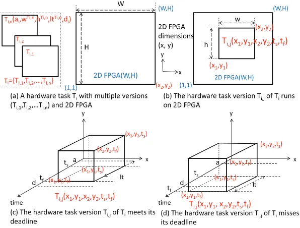
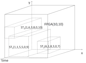
A 2D dynamically reconfigurable FPGA, denoted by FPGA (W,H) as illustrated inFig. 1, containsWHreconfigurable hardware units arranged in a 2D array, where each element of the array can be connected with other element(s) using the FPGA interconnection network. The reconfigurable unit located inithposition in the first coordinate (x) andjthposition in the second coordinate (y) is identified by coordinate (i,j), counted from the lower-leftmost coordinate (1, 1), where 16i6Wand 16j6H.
A hardware taskTiwithnmultiple hardware versions, denoted byTi= {Ti,1,Ti,2,. . .,Ti,n}, arrives to the system at arrival timeaiwith deadlinedias shown inFig. 1. Each version requires a region of sizewhin the 2D FPGA (W,H) during its life-timelt; it can be represented as a 3D box inFig. 1(c) or (d). We call this as a3D representation of the hardware task. We define
lt= rt+etwherertis the reconfiguration time andetis the execution time of the task.wandhare the task width and height where 16w6W, 16h6H.
Online task scheduling and placement algorithms targeting 2D FPGAs with multiple selectable hardware versions have to choose the best hardware implementation on-the-fly at runtime among those available hardware variants and find a region of hardware resources inside the FPGA for running the chosen hardware version for each arriving task. When there are no available resources for allocating the hardware task at its arrival timea, the algorithm has to schedule the task for future execution. In this case, the algorithm needs to find the starting timetsand the free region (withlower-leftmost corner (x1,y1) andupper-rightmost corner(x2,y2)) for executing the task in the future. The running or scheduled task is denoted asT(x1,y1,x2,y2,ts,tf), wheretf=ts+ltis the finishing time of the task. The hardware task meets its deadline iftf6d. We also call thelower-leftmost cornerof a task as theoriginof that task.
The goals of any scheduling and placement algorithm are to minimize the total number of hardware tasks that miss their deadlines and to keep the runtime overhead low by minimizing algorithm execution time. We express thedeadline miss ratio
as the ratio between the total number of hardware tasks that miss their deadlines and the total number of hardware tasks arriving to the system. Thealgorithm execution timeis defined as the time needed to schedule and place the arriving task.
4. System model
In this article, each hardware task with multiple hardware versions can arrive at any time and its properties are unknown to the system beforehand. This models real situations in which the time when the user requests system resources for his/her usage is unknown. As a result, the envisioned system has to provide support for runtime hardware tasks placement and scheduling since this cannot be done statically at system design time. To create multiple hardware variants, it can be done
by controlling the degree of parallelism[10–15], implementing hardwares using different architectures[16,17]and algo-rithms[18,19]. Some of known techniques to control the degree of parallelism are loop unrolling with different unrolling factors[10–13], recursive variable expansion (RVE)[14], and realizing hardwares with different pipeline stages[15].
Similar to other work, we assume that each hardware version requires reconfigurable area with rectangular shape and can be placed at any location on the reconfigurable device. Our task model includes all required reconfigurable units and interconnect resources. Each hardware version is first designed using a hardware description language and after that is placed and routed by commercial FPGA synthesis Computer-Aided Design (CAD) tools to obtain functionally equivalent mod-ules that can replace their respective software versions. At this step of the design process we can use the synthesis results to extract the task sizes for the used FPGA fabric. The output of the synthesis is the configuration bitstream file. The reconfig-uration time of the targeted technology is the elapsed time needed to load the bitstream file to the device using its integrated configuration infrastructure. The two key ingredients are the configuration data size (the bitstream length in number of bits) and the throughput of the internal FPGA configuration circuit. As an example, theInternal Configuration Access Port(ICAP) [29] of Virtex 4 FPGAs from Xilinx can transport 3200 million bits/second and will load a bitstream of size 51 Mbits in 15.9 ms. The last parameter, the task execution time is specified by the time needed to process a unit of data (referred
as:Execution Time Per Unit of Data, ETPUD) and the overall data size to be processed (i.e. how much data need to be
pro-cessed). Please note that for some applications, the task execution time is also dependent on the exact data content (e.g., as in the case of Viterbi andContext-Adaptive Binary Arithmetic Coding(CABAC)). In such applications, even when processing the same amount of data, the elapsed time will be different when the input data content changes. To address data dependent task execution times, we envision two solutions:worst case execution timescenario andnotification on task completion hard-ware support.
In this article, we assume the worst case execution time scenario in which we use the task execution time when process-ing the worst case input data content. In such scenario, it is possible that the actual task completion can happen earlier than the scheduled completion time resulting in idle times that can not be used by the algorithm. In addition, such tasks will cause additional wasted area that cannot be utilized immediately by other hardware tasks. In such non-optimal scenario, however, the overall computing system will operate correctly. Please note that the chosen scenario is the worst case in re-spect to the proposed placement and scheduling algorithm due to the introduced overheads in task execution time and wasted area. The second solution requires dedicated hardware support for feedback signaling when the running tasks com-plete, however, as mentioned earlier this can additionally improve the overall system performance. Some existing systems already have the necessary ingredients required to implement such support. For example, in the Molen architecture[30], the sequencer is aware of the hardware task start and completion timing. The only necessary extension in this case is to provide a way to pass this information to the scheduling and placement algorithm and make it aware of running tasks completion. With this knowledge, the algorithm can make data content dependent tasks scheduling more efficient. This approach is out-side of the scope of this work without loosing generality of our proposal. Even more the selected worst case execution sce-nario is less beneficial for the scheduling and placement algorithm presented in this study. We are strongly convinced that both types of systems will be able to benefit from the proposed algorithms.
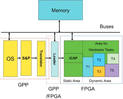
The assumed overall system model used in our study is sketched inFig. 2consisting of two main devices: the general-purpose processor (GPP) and the reconfigurable device (e.g. FPGA). All hardware task bitstream images are available in a repository resuming in the main memory (not explicitly shown on the figure) and can be requested by any running appli-cation on the GPP by using a dedicated operating system (OS) call. In response to such request, the OS will invoke the sched-uling and placement algorithm (S&P) to find the best location on the FPGA fabric for the requested hardware task. Once appropriate location is found, the Translator will resolve the coordinates by transforming the internal, technology indepen-dent model representation to the corresponding low level commands specific for the used FPGA device. The Loader reads the
task configuration bitstream from the repository and sends it to the internal configuration circuit, e.g., ICAP in case of Xilinx, to partially reconfigure the FPGA at the specific physical location provided by the Translator. After reconfiguring the FPGA fabric the requested hardware task execution is started immediately to avoid idle hardware units on the reconfigurable fab-ric. When the hardware area is fully occupied, the scheduling and placement algorithm (S& P) schedules the task for future execution at predicted free area places at specific locations and specific starting times. The Loader can be implemented at either the GPP as OS extension or in the Static Area of the FPGA. If the Loader is implemented in the GPP, the communication between the Loader to the ICAP is performed using the available off-chip connection. For implementations in the FPGA, the Loader connects to the ICAP internally. Similar to[31], dedicated buses are used for the interconnect on chip. Those buses are positioned at every row of the reconfigurable regions to allow data connections between tasks (or tasks and Inputs/Out-puts(I/Os)) regardless of the particular task sizes.
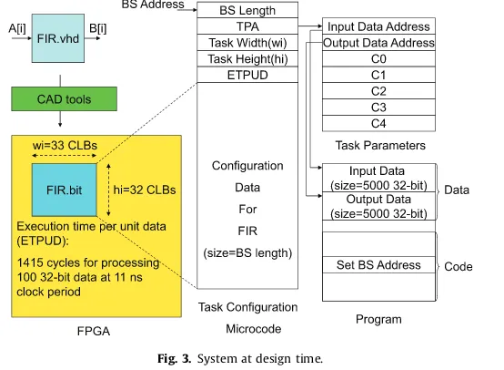
To illustrate the above processes at different stages of the system design and normal operation, we will use a simple example of hardware task creation as depicted inFig. 3. The hardware task in our example is a simple finite impulse response (FIR) filter. The task consumes input data from array A[i] and produces output data stored in B[i], where
B[i] =C0A[i] +C1A[i+ 1] +C2A[i+ 2] +C3A[i+ 3] +C4A[i+ 4] and all data elements are 32 bits wide. The task implementation described using a hardware description language (HDL) (FIR.vhd) is synthesized by commercial CAD tools that produce the partial bitstream file (FIR.bit) along with the additional synthesis results for that task. The bitstream con-tains the configuration data that should be loaded into the configuration memory to instantiate the task at a certain location on the FPGA fabric. The synthesis results are used to determine the rectangle area consumed by the task in terms of config-urable logic blocks (CLBs) specified by the width and the height of the task. In our example, the FIR task width is 33 and the task height 32 CLBs for Xilinx Virtex-4 technology. Based on the synthesis output we determine the tasks reconfiguration times. Please note, that in a realistic scenario one additional design space exploration step can be added to steer task shapes toward an optimal point. At such stage, both, task sizes and reconfiguration times are predicted by using high-level models as the ones described in[32]in order to perform quick simulation of the different cases without the need of synthesizing all of the explored task variants. For example in Virtex-4 FPGA technology from Xilinx, there are 22 frames per column and each frame contains 1312 bits. Therefore one column uses 221312 = 28,864 bits. Since our FIR hardware task requires 33 CLBs in 2 rows of 16 CLBs totaling in 32 CLBs, we obtain a bitstream with 33228,864 = 1,905,024 bits. Virtex-4 ICAP can send 32-bit data every 100 MHz clock cycle, hence, we can calculate the reconfiguration time as 1,905,02410/32 = 595,320 ns. Next, the FIR task is tested by the designer to determine how fast the input data can be processed. For our example from Fig. 3, the task needs 1415 cycles to process 100, 32-bit input data elements at 11 ns clock period making its ETPUD 141511 = 15,565 ns per 100, 32-bit unit data. Based on the above ETPUD number, we can compute the task execution time for various input data sizes. In our example, there are 5000, 32-bit input data elements that have to be processed by the FIR hardware task. Therefore, the expected execution time of our FIR task is (5000/100)15,565 = 778,250 ns (778 ms). The configuration data, together with task specific information, forms aTask Configuration Microcode(TCM) block as shown in the upper part ofFig. 3. TCM is pre-stored in memory at the Bitstream (BS) Address. The first field, the BS length represents the size of the configuration data field. This value is used by the Loader when the task is fetched from memory. The task parameter address (TPA) is needed to define where the task input/output parameters are located. InFig. 3, the task param-eters are the input and output data locations, the number of data elements to be processed and the FIR filter coefficients (C0– C4). The input data address gives the location where the data to be processed remains. The location where the output data should be stored is defined by the output data address.
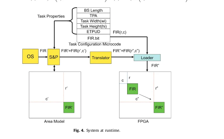
During runtime, when the system needs to execute the FIR hardware task on the FPGA, the OS invokes the scheduling and placement algorithm (S&P) to find a location for it (shown as example, inFig. 4). From the TCM the algorithm gets the task properties information: task width, task height, reconfiguration time, and its execution time. Based on the current state of the used area model, the algorithm searches for the best location for the task. When the location is found (in this example:r0 andc0), the task is placed in the area model and its state is updated as shown on the left side of the figure. The Translator converts this location into real physical location on the targeted FPGA. In the bitstream file (FIR.bit), there is information about the FPGA location where the hardware task was pre-designed (in this figure: r and c). By modifying this information at runtime, the Loader partially reconfigures the FPGA through the ICAP (by using the technology specific commands) at the location obtained from the Translator (r00andc00in this example). By decoupling our area model from the fine-grain details of the physical FPGA fabric, we propose an FPGA technology independent environment, where different FPGA vendors, e.g., Xi-linx, Altera, etc, can provide their consumers with full access to partial reconfigurable resources without exposing all of the proprietary details of the underlying bitstream formats. On the other side, reconfigurable system designers can now focus on partial reconfiguration algorithms without having to bother with all low-level details of a particular FPGA technology.
5. Algorithm
In this section, we discuss the proposed algorithm in detail. We first present the pertinent preliminaries along with some essential supported examples that will serve as foundation to more clearly describe the key mechanisms of the proposed algorithm. Then, to clearly illustrate the basic idea of our proposal, we show a motivational example. Finally, we describe the process of building our proposed strategy based on previous foundational discussions.
5.1. Preliminaries
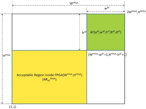
Definition 1. The acceptable region inside FPGA (WFPGA,HFPGA) of an arriving hardware taskAT(aAT,wAT,hAT,ltAT,dAT), denoted asARFPGAAT , is a region where the algorithm can place theoriginof the arriving taskATwithout exceeding the FPGA boundary.
Therefore, the acceptable region has the lower-leftmost corner (1, 1) and upper-rightmost corner (WFPGAwAT+ 1,HFPGA hAT+ 1) as illustrated inFig. 5.
Definition 2. The conflicting region of an arriving hardware taskAT(aAT,wAT,hAT,ltAT,dAT) with respect to a scheduled task
ST xST
1;yST1;xST2;yST2;tSTs ;t ST f
, denoted asCRSTAT, is the region where the algorithm cannot place theoriginof the arriving task
ATwithout conflicting with the corresponding scheduled taskST. The conflicting region is defined as the region with its lower-leftmost corner max1;xST
1 wATþ1
;max 1;yST1 h
AT þ1
and upper-rightmost corner ðmin xST 2;W
FPGA
wATþ1Þ;min yST 2;H
FPGA
hATþ1
Þas presented inFig. 6.
Definition 3. An arriving task AT(aAT,wAT,hAT,ltAT,dAT) at position xAT 1 ;yAT1
is said to have a common surface with
FPGA(WFPGA,HFPGA) boundary if xAT 1 ¼1
_ xAT
1 ¼W FPGA
wATþ1
_ yAT 1 ¼1
_ yAT
1 ¼H FPGA
hATþ1
.
Definition 4. The compaction value withFPGA(WFPGA,HFPGA) boundary for an arriving taskAT(aAT,wAT,hAT,ltAT,dAT), denoted asCVAT
FPGA, is the common surfaces between FPGA boundary and the arriving task.
Example 1. Let us computeCVAT
FPGAat position (1,1) of an example inFig. 7. The arriving taskAT(a
AT,wAT,hAT,ltAT,dAT) at
posi-tion (1, 1) has two common surfaces (i.e. bottom and left surfaces) withFPGA(WFPGA,HFPGA) boundary. Therefore, theCVATFPGAis the sum area of these surfaces,CVAT
FPGA= area of bottom surface + area of left surface =w
ATltAT+hATltAT= (wAT+hAT)ltAT.
Definition 5. An arriving task AT(aAT,wAT,hAT,ltAT,dAT) at position ðxAT
1;yAT1Þ is said to have a common surface with
ST xST
1;yST1;xST2;yST2;tSTs ;tSTf
if tST f >tATs
^ ðtST s 6tATs Þ
^ : yAT 1 þh
AT <yST1
_ yAT 1 >yST2 þ1
_ xAT
1 þwAT<xST1
_
xAT 1 >xST2 þ1
Þ.
Definition 6. The compaction value with an scheduled taskST xST
1;yST1;xST2;yST2;tSTs ;tSTf
for an arriving taskAT(aAT,wAT,hAT,
ltAT,dAT), denoted asCVATST, is the common surface between the scheduled task and the arriving task.
Definition 7.The total compaction value of an arriving taskAT(aAT,wAT,hAT,ltAT,dAT), denoted asTCVAT
ST, is the sum ofCV AT ST with all scheduled tasks that have the common surface with the arriving task AT.
Fig. 5.An example of acceptable region insideFPGA(WFPGA
,HFPGA
) of an arriving taskAT(aAT
,wAT
,hAT
,ltAT
,dAT
).
Fig. 6.An example of the conflicting region of an arriving taskAT(aAT
,wAT
,hAT
,ltAT
,dAT
) with respect to a scheduled taskST xST
1;yST1;xST2;yST2;t ST s;t
ST f
Example 2. Let us computeCVAT
ST at position as illustrated inFig. 8. The arriving taskAT(a
AT,wAT,hAT,ltAT,dAT) at that position
has the common surface (i.e. between the right surface of the scheduled task ST and the left surface of the arriving task AT). Therefore, theCVAT
ST is the area of this surface,CV AT
Definition 8. The finishing time difference with a scheduled taskST xST
1;yST1;xST2;yST2;tSTs ;tSTf
if the arriving task AT has a common surface with the scheduled task ST.
Definition 9. The total finishing time difference of an arriving taskAT(aAT,wAT,hAT,ltAT,dAT), denoted asTFTDAT
ST, is the sum of
FTDATST with all scheduled tasks that have the common surface with the arriving task AT.
Definition 10. The hiding value of an arriving task AT(aAT,wAT,hAT,ltAT,dAT) at position xAT
ST, is formulated as HV
AT
as illustrated in Fig. 9(a). In this example tST
f ¼tATs , therefore, HV
as illustrated in Fig. 9(b). In this example tAT
f ¼tSTs , therefore, HV AT
ST ¼max minð
Fig. 7.An example of the compaction value withFPGA(WFPGA
,HFPGA
) boundary for an arriving taskAT(aAT
,wAT
,hAT
,ltAT
,dAT
) at position (1, 1).
Fig. 8.An example of the compaction value with scheduled taskST xST
xAT scheduled tasks that satisfy the tST
f ¼t ing time for the arriving task AT placed on the FPGA at the potential position columniand rowj.
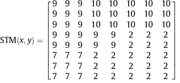
Example 5. Let us compute the starting time matrix of an arriving taskAT(2, 3, 3, 5, 10) onFPGA(10, 10) inFig. 10. The size of STM(x,y) is (WFPGAwAT+ 1)(HFPGAhAT+ 1) = (103 + 1)(103 + 1) = 88. Let us assume that the current time is 2 time units.
To computer the value of STM(1, 1), we have to place the arriving task on the FPGA at the potential position column 1 and row 1. Since the size of the arriving task is 33, if we place this arriving task at position (1, 1), we need to use reconfigurable units from columns 1 to 3 and rows 1 to 3. In this current time, these needed reconfigurable units for the arriving task are being used by the scheduled taskST1. Therefore, the earliest starting time at position (1, 1) for the AT will be after theST1 terminates at time unittST1
f ¼9, STM(1, 1) = 9.
To computer the value of STM(1, 4), we have to place the arriving task on the FPGA at the potential position column 1 and row 4. If we place this arriving task at this position, we need to use reconfigurable units from columns 1 to 3 and rows 4 to 6. In this current time, these needed reconfigurable units for the arriving task are being used partially by the scheduled taskST1
(a)
(b)
Fig. 9.Examples of the hiding value of an arriving taskAT(aAT
,wAT
with a scheduled taskST xST
1;yST1;xST2;yST2;tSTs;tSTf
.
(columns 1–3 and rows 4–5) andST3(columns 1–3 and row 6). Therefore, the earliest starting time at this position for the AT
Using the same method as above computations, we can compute the values of all elements in the STM(x,y) matrix to produce the STM(x,y) matrix as following:
STMðx;yÞ ¼
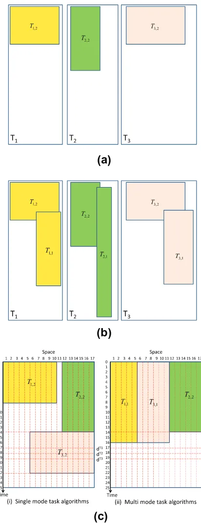
The basic idea of our proposal is to use as least as possible reconfigurable resources to meet the deadline constraint of each incoming task. In order to clearly describe the main idea of our proposal, we use a motivational example (Fig. 11) which sketches the scheduling and placement of a hardware task set by single mode task algorithms and multi mode task algo-rithms. In this figure, the length and the width of a rectangle represents the required reconfigurable area of FPGA to run the corresponding task and its lifetime of staying on this fabric.
Fig. 11(a) shows a simple hardware task set that is composed of 3 single mode hardware tasks (T1,T2, andT3); each task has only one hardware version (i.e.T1,2,T2,2, orT3,2). Unlike the single mode hardware task set, each hardware task in the multi mode hardware task set is composed of a variety of different hardware implementations as illustrated inFig. 11(b). In this instance, each task has two hardware versions depending on the desired performance (e.g. taskT1with its two hard-ware versionsT1,1andT1,2). Each version has its own speed with required reconfigurable area for running it on FPGA. For example, with more required area, versionT1,2runs faster than versionT1,1. Let us assume that these three tasks arrive to the system at timet= 0 and the FPGA has 17 free reconfigurable units at that time. Single mode task algorithms allocate task
T1,2at the left side of the FPGA (units 1–10), starting fromt= 0 and ending att= 8; taskT1meets its deadline as shown in Fig. 11(c)-i. Instead of usingT1,2, multi mode task algorithms decide to run taskT1using a different hardware versionT1,1 with slower speed but less required area, which still can meet its deadline constraint as illustrated inFig. 11(c)-ii. The idea is that this saved area can be used later by other tasks. For taskT2, the multi mode algorithms do not use a smaller hardware version (T2,1), because this hardware version cannot meet the deadline constraint of taskT2. Therefore, the larger hardware versionT2,2is chosen for running taskT2that can satisfy the deadline constraint as shown inFig. 11(c)-ii. Since single mode task algorithms is paralyzed by its inflexibility of choosing the best solution to run tasks in reconfigurable fabric, almost all reconfigurable area at timet= 0 is occupied by other tasks (only left 1 unit), taskT3cannot be operated at timet= 0. There-fore, it needs to be scheduled later, in this case att= 14, after the termination ofT2,2. As a consequence, it cannot meet its deadline as shown inFig. 11(c)-i. This miss deadline case can be eliminated if we use multi mode algorithms. In the multi mode algorithm, since it saves a lot area during scheduling previous task (in this case taskT1), free area at timet= 0 still big enough for allocating hardware versionT3,1. As a result, the deadline constraint ofT3is met as illustrated inFig. 11(c)-ii.
5.3. Pseudocode and analysis
By orchestrating all heuristics introduced earlier, we develop the proposed strategy, called aspruning moldable (PM); the pseudocode of the algorithm is shown inAlgorithm 1. To reserve more free area for future incoming tasks, when a new task with multiple hardware versions AT arrives to the system, the algorithm tries to choose the slowest hardware task first in which the required reconfigurable area is minimized as shown in line 1. With respect to this chosen hardware implemen-tation, the starting time matrix STM(x,y) adopted fromDefinition 12is built as shown in line 2. This step will be explained further later when we are talking aboutAlgorithm 2. The key idea of this step is to empower the algorithm to always choose the earliest starting time for every single arriving task. In line 3, the algorithm finds thesmallest starting time(SST) from STM(x,y), which is the smallest value in the matrix. This SST is the earliest time we can schedule the chosen hardware task, which is optimized in time direction. This best position in time will be utilized later in line 4 to steer the algorithm in making decision of the best hardware variant. This result also will be used further to steer the algorithm to choose the best position not only in time but also in space directions later in lines 8–15 as our goals.
the current solution. If the current solution cannot satisfy the deadline constraint of the respective task (i.e.tAT f >d
AT ) and all implemented hardwares have not been tried yet, the algorithm switches to the faster hardware variant with more hardware resources for finding a better solution (lines 5–6) looping back to line 2 for computing a new STM(x,y) matrix with respect to the new hardware version. Otherwise, it skips lines 5–6 and proceeds to line 8 to start finding the best solution among best candidates.
To significantly reduce runtime overhead, the search space should be minimized by avoiding any unnecessary search. For that purpose, the algorithm is armed with an ability to prune search space. With this ability, it is not necessary to check all
(a)
(b)
(c)
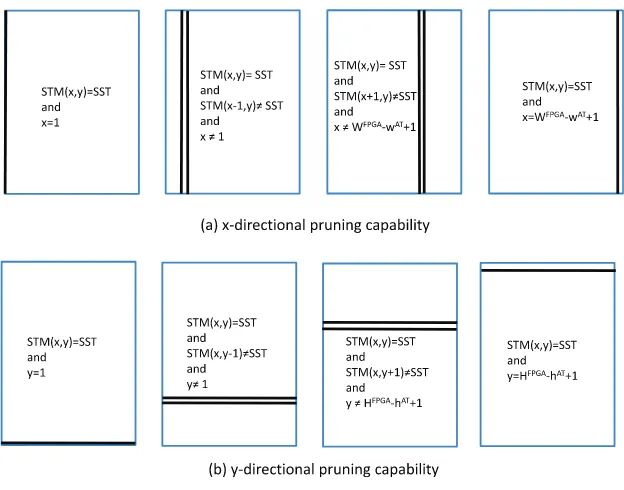
elements in STM(x,y) matrix for searching the best position for each incoming task. It only needs to check the potential positions (line 8) that can satisfy thepruning constraints(line 9) using its2D-directional pruning capability(Fig. 12) from the best positions steered by SST from line 3. Line 8 gives the algorithm an ability to choose the only best potential positions from all positions in STM(x,y) matrix in time direction. The search space is pruned further by only searchingunrepeated adjacent elements in x direction ((STM(x,y) = SST^STM(x1,y)–SST^x–1)_(STM(x,y) = SST^STM(x+ 1,y)–SST^
x–WFPGAwAT+ 1)) and y direction ((STM(x,y) = SST^STM(x,y1)–SST^y–1)_(STM(x,y) = SST^STM(x,y+ 1)– SST^y–HFPGAhAT+ 1)) and FPGA boundary adjacent elements ((STM(x,y) = SST^x= 1)_(STM(x,y) = SST ^x=
WFPGAwAT+ 1)_(STM(x,y) = SST^y= 1)_(STM(x,y) = SST^y=HFPGAhAT+ 1)) within the area dictated by line 8 as shown inFig. 12. By doing this, the algorithm can find the best solution for each arriving task faster as will be shown later in the evaluation section.
After pruning the searching space, the algorithm needs to find the best position for the incoming task among best poten-tial positions produced by previous pruning processes. To do this, the variable
a
ATis introduced in line 12, which is the sum ofCVATFPGA(Definition 4),TCVAT
ST(Definition 7), andTHV AT
ST(Definition 11). This new variable is used in line 13 to advise the algo-rithm to find the best solution. The computation ofCVAT
FPGA; TCV AT ST; THV
AT
ST, andTFTD AT
ST is done in lines 10–11. In line 13, the algorithm chooses the best position for the chosen hardware version based on its current availability of hardware resources, resulting the best position both in space and time.
Algorithm 1. Pruning Moldable (PM)
1: choose the slowest hardware version 2: build STM(x,y) (seeAlgorithm 2) 3: find the smallest starting time (SST) 4:iftAT
f >d AT
andall alternative hardware versions have not been tried 5: switch to the faster hardware version
6: go to line 2 7:end if
8:forall positions with SSTdo
9: if(STM(x,y) = SSTandx= 1)or
(STM(x,y) = SSTandSTM(x1,y)–SSTandx–1)or (STM(x,y) = SSTandSTM(x+ 1,y)–SSTandx–WFPGA
wAT+ 1)or (STM(x,y) = SSTandx=WFPGAwAT+ 1)or
(STM(x,y) = SSTandy= 1)or
(STM(x,y) = SSTandSTM(x,y1)–SSTandy–1)or
(STM(x,y) = SSTandSTM(x,y+ 1)–SSTandy–HFPGAhAT+ 1)or (STM(x,y) = SSTandy=HFPGAhAT+ 1)
10: computeCVATFPGA(seeAlgorithm 3)
11: computeTCVAT ST; THV
AT
ST, andTFTD AT
ST (seeAlgorithm 4)
12:
a
AT¼CVATFPGAþTCVATSTþTHVATST13: choose the best position (seeAlgorithm 5) 14: end if
15:end for
16: update linked lists (seeAlgorithm 6)
The detail information of how the algorithm builds the STM(x,y) matrix is shown in Algorithm 2. The aim is to quickly find the earliest time for launching each newly-arrived task by inspecting its acceptable and conflicting regions (Definitions 1 and 2). The constructing of STM(x,y) matrix consists of an initialization and a series of updating opera-tions. Two linked lists, denoted as the execution list EL and the reservation list RL, are managed by the algorithm. The EL keeps track of all currently running tasks on FPGA, sorted in order of increasing finishing times; the RL records all scheduled tasks, sorted in order of increasing starting times. Initially, there are no tasks in the lists (EL =;and RL =;). Each element in the lists holds the information of the stored task: the lower-left corner (x1,y1), theupper-right corner
Definition 2. Hence, by inspecting the acceptable and conflicting regions, it is not necessary to check the state of each reconfigurable unit in the FPGA. Not all elements in this overlapped area need to be updated to the finishing time of scheduled tasktST
f ; only elements that have values less thantSTf need to be updated (line 9). The STM(x,y) matrix also can be influenced by tasks in the reservation list RL if RL–;(line 15). Similar like updating STM(x,y) by the EL, the area defined byCRSTATneeds to be evaluated (lines 16–17). Besides checking the finishing time, the updating of STM(x,y) by the RL needs to check the starting time of scheduled tasks as well (line 18). This process needs to ensure that only the ele-ment overlapped in space and time with scheduled tasks needs to be updated (line 19).
Let us use this algorithm to compute STM(x,y) matrix inExample 5andFig. 10. FromFig. 10, since the current time is two time units, all tasks in the figure are under operation; as a result, all tasks are recorded in the execution list sorted in order of increasing finishing times (i.e.EL= {ST3,ST1,ST2}) and there is no task in the reservation list. Since theRL=;, the execution of lines 15–23 does not affect the STM(x,y) matrix. After execution of lines 1–5, the STM(x,y) will be filled with the arrival time of the incoming task AT(2, 3, 3, 5, 5, 10) (i.e.aAT= 2 time units); hence, the matrix will be as following:
STMðx;yÞ ¼
Next, the algorithm proceeds to lines 6–14, updating STM(x,y) with respect to scheduled tasks in the execution list
Subsequently, using the same method, the algorithm needs to update the STM(x,y) affected byST1(i.e.tSTf 1¼9 time units)
Finally, again using the same strategy, the algorithm proceeds to update the STM(x,y) affected byST3(i.e.tSTf 3¼10 time units) as following:
Algorithm 2. Building STM(x,y) matrix
The pseudocode to compute compaction value with FPGA boundary, denoted asCVAT
FPGA and adopted fromDefinition 4, is shown inAlgorithm 3. The motivation of this heuristic is to give awareness of FPGA boundary to the algorithm. The
CVATFPGA is zero (line 1) if the position of the arriving task does not satisfy the condition defined inDefinition 3(lines 2, 4, and 6); in this case, the arriving tasks does not have any common surface with FPGA boundary. The initialization of
CVAT
FPGA is presented in line 1; it is set to zero. The condition in line 2 is satisfied if two surfaces of the arriving task in 3D representation touch the FPGA boundary, i.e. the arriving task is allocated at one of the corners of FPGA; in this situation, theCVATFPGA is equal to the sum of area of the common surfaces, (w
AT+
hAT)ltATas shown in line 3. Please note that the 3D representation of hardware task has been discussed in Section3. The satisfaction of condition either in line 4 or 6 means that the arriving task has only one common surface with FPGA boundary; here, theCVATFPGA can be calculated as the area of that common surface which is eitherhAT ltAT (line 5) orwATltAT(line 7).
Let us use this algorithm to computeCVAT
FPGAinExample 1andFig. 7. First, in line 1, the algorithm initializesCV AT
FPGAto zero. Since the potential position is (1,1) (i.e.xAT
1 ¼1 andyAT1 ¼1), the condition in line 2 is satisfied. As a result, the algorithm proceeds from line 2 to line 3 and ends up to line 8. Therefore, theCVATFPGAis computed asCV
AT
FPGA¼ ðwATþh AT
Þ ltAT.
Algorithm 3. ComputingCVATFPGA
1:CVATFPGA¼0
Algorithm 4shows the pseodocode of computingTCVATST (Definition 7),THV AT
ST (Definition 11), andTFTD AT
ST (Definition 8). The heuristicTCVAT
ST is required to equip the algorithm to pack tasks in time and space. To give the algorithm an awareness of ‘‘blocking effect’’, the heuristicTHVATSTis added to it. The last employed heuristicTFTD
AT
STsteers the algorithm to group hard-ware tasks with similar finishing times; as a result, more adjacent tasks depart from FPGA at the same time, creating the larger free area during deallocation. The initialization is done in lines 1–3; all variables are set to zero. To compute the values of these variables, the algorithm needs to check all scheduled tasks in linked lists RL and EL (line 4) that can affect their val-ues. Not all scheduled tasks in linked lists need to be considered for computation, only tasks touched by the arriving task. For example inFig. 13, the considered tasks are only three tasks (T12,T15andT16).Definition 5discussed before is implemented
in line 5 in this algorithm. IfDefinition 5is not satisfied, theTCVATST andTFTD AT
ST are zero. The scheduled task and the arriving task can have a common surface in one of different ways as shown in lines 6–30. Based onDefinitions 6 and 7, theTCVAT
STis computed as the sum of common surface by its considered tasks; each added value has two components (commonality in space and time). For example, in line 7, the commonality in space is computed aswATwhile the commonality in time is rep-resented asmin ltAT; tSTf tAT
s
. As far as there is a common surface between the scheduled task and the arriving task, the
FTDAT
ST is added cumulatively toTFTD AT
ST, which is the finishing time difference between the arriving task and considered tasks as defined inDefinitions 8 and 9. The computation of total hiding valueTHVATSTofDefinitions 10 and 11is applied in lines 31– 33; it only has value if one of these conditions is satisfied: (1) the arriving task is scheduled immediately once the scheduled task is terminated (tST
f ¼tATs , e.g. the arriving task AT and taskT12inFig. 13) or (2) the termination of arriving task is right
away before the start of the scheduled task tAT f ¼tSTs
as shown in line 31.
Let us computeTCVATST; THV AT
ST, andTFTD AT
STinFig. 8using this algorithm. In this situation, the execution list is filled by one scheduled taskST xST
1;yST1;xST2;yST2;tSTs ;tSTf
(i.e.EL¼ STðxST
1;yST1;xST2;yST2;tSTs ;tSTf Þ
n o
); whereas the reservation list is empty. All
computation variables is initialized to zero in lines 1–3 (i.e.TCVATST ¼0; THVAT
ST ¼0; TFTD
AT¼0). In line 4, the algorithm
con-siders the scheduled task in EL,STðxST
1;yST1;xST2;yST2;t ST s ;t
ST
f Þ. Since the condition in line 5 and line 9 are satisfied, the algorithm proceeds to lines 10-11 and ends up at line 34. In line 10, the total compaction value with scheduled tasks is updated,
Table 1
Time complexity analysis of Pruning Moldable (PM) algorithm.
Line(s) Time complexity
1 O(1)
2 O(WHmax(NET,NRT))
3 O(WH)
4–7 O(nWHmax(NET,NRT))
8–15 O(WHmax(NET,NRT))
16 O(max(NET,NRT))
Total O(nWHmax(NET,NRT))
TCVAT
line 11, the total finishing time difference is renewed, TFTDAT ST¼TFTD
AT
STþ jtATf tSTf j ¼0þ jtfATtSTf j ¼ jtATf tSTf j. Since the algorithm skips lines 31-33, the total hiding value becomes zero.
To complete our discussion, let us computeTCVAT algorithm executes lines 1–3, the initialization. In figure (a), since the arriving task is started right away after the scheduled task (i.e.tST
f ¼tATs ), the condition in line 5 cannot be satisfied; the algorithm proceeds to line 31. The algorithm skips lines 6-30; hence,TCVAT
ST ¼0 andTFTD AT
ST¼0. In line 31, the condition oftSTf ¼tATs is satisfied; therefore, the total hiding value is updated for figure (a), THVAT
ST¼THV
in figure (b), since the scheduled task is started right away after the arriving task (i.e.tAT f ¼t
ST
s ) and the starting time of scheduled task is more than the starting time of arriving task (i.e.tST
s >tATs ), the condition in line 5 cannot be satisfied; the algorithm proceeds to line 31. The condition in line 31 is satisfied bytAT
f ¼tSTs . As a result, the total hiding value is updated for figure (b),THVAT
ST ¼THV algorithm skips lines 6-30 for figure (b); hence,TCVAT
ST ¼0 andTFTD AT ST ¼0.
The pseudocode of choosing the best position among best potential candidates is depicted inAlgorithm 5. The goals of this algorithm are to maximize
a
ATand minimizeTFTDATST. If both these goals cannot be satisfied at the same time, the heu-ristic used here is to prioritize maximizing
a
ATthan minimizingTFTDATST. In line 1, if the checking position produces highera
AT and lowerTFTDATST than the current chosen position, the checking position is selected as a new current chosen position, replacing the old one (lines 2–3) and updating
a
max(line 4) andTFTDminST (line 5). Since the heuristic is to favor maximizing
a
ATthan minimizingTFTDATST, the algorithm is designed to change the chosen position (lines 7–8) and update itsa
max(line 9) as far asa
ATcan be maximized (line 6). In line 10, if both conditions in lines 1 and 6 cannot be satisfied, the only condition that can change the decision is by minimizingTFTDATST while preserving
a
maxat its highest value. This heuristic guides the
algorithm to choose the position with the highest
a
maxthat produces the lowestTFTDATST.Algorithm 5. Choosing the best position
1:if
a
AT>a
maxandTFTDATST <TFTDminST thenAlgorithm 6shows how the algorithm updates its linked lists (i.e. EL and RL). If the arriving task can be started immedi-ately at its arrival time (i.e.SST=aAT), it is added in the execution list EL, sorted in order of increasing finishing times (line 2). The algorithm needs to schedule this incoming task to run it in the future if there is no available free reconfigurable resources for it at its arrival time (line 3) by adding it to the reservation list RL (line 4); the addition is sorted in order of increasing starting times. During the updating (lines 6–11), each element of the EL is checked by comparing its finishing time with the current time for removing it from the list after finishing executed in the FPGA. Tasks in the RL are moved to the EL if they are ready to be started running on the FPGA during this updating.
Table 2
Some examples of implemented hardware tasks (etifor 100 operations,rtiat 100 MHz).
Algorithm 6. Updating the linked lists
1:ifSST=aATthen 2: add the AT to the EL 3:else
4: add the AT to the RL 5:end if
6:ifRL–;then
7: update RL 8:end if
9:ifEL–;then
10: update EL 11:end if
The worst-case time complexity analysis of the PM is presented inTable 1. In whichW,H,NET,NRT, n are the FPGA width and height, the number of executing tasks in the execution list, the number of reserved tasks in the reservation list and the number of hardware versions for each task, respectively.
6. Evaluation
In this section, we discuss the evaluation of the proposed algorithm in detail. We first detail the experimental setup. Then, based on the prepared setup, we present the evaluation of our proposal with synthetic hardware tasks. Finally, to complete the discussion, we discuss the evaluation of the proposal with real hardware tasks.
6.1. Experimental setup
To evaluate the proposed algorithm, we have built a discrete-time simulation framework in C. The framework was com-piled and run under Windows XP operating system on Intel(R) Core(TM)2 Quad Central Processing Unit (CPU) Q9550 at 2.83 GHz Personal Computer (PC) with 3GB of Random-Access Memory (RAM). We model a realistic FPGA with 116 columns and 192 rows of reconfigurable units (Virtex-4 XC4VLX200). To better evaluate the algorithm, (1) we modeled realistic ran-dom hardware tasks to be executed on a realistic target device; (2) we evaluated the algorithm not only with synthetic hard-ware tasks but also with real hardhard-ware tasks; and (3) since the algorithm needs to make a decision at runtime, we measured the algorithm performance not only in terms of scheduling and placement quality, which is related to its deadline miss ratio, but also in terms of runtime overhead. Since the algorithms are online, the information of each incoming task is unknown until its arrival time. The algorithm is not allowed to access this information at compile time. Every task set consists of 1000 tasks, each of which has two hardware versions with its own life-time and task size. We assume the task width of the slowest hardware implementation is half of its original variant, running two times slower than its original one. All results are pre-sented as an average value from five independent runs of experiments for each task set. Therelative deadlineof an arriving task is defined asrdAT=dATltATaAT. It is also randomly generated with the first number and the second number shown in the x-axis of the experimental results as the minimum and maximum values, respectively. Furthermore, our scheduling scheme is non-preemptive – once a task is loaded onto the device it runs to completion.
The proposed algorithm is designed for 2D area model. Therefore for fair comparison, we only compare our algorithm with the fastest and the most efficient algorithms that support 2D area model reported in the literature. Since the RPR[24], the Communication-aware[25], the Classified Stuffing[21], the Intelligent Stuffing were designed only for 1D area model, we do not evaluate them in this simulation study. In[20], the Stuffing was shown to outperform the Horizon; hence we do not include the Horizon in comparison to our proposal. The CR algorithm was evaluated to be superior compared to the ori-ginal 2D Stuffing[20]and the 2D Window-based Stuffing[26]in[27]. For that reason, we do not compare our algorithm to the original 2D Stuffing and the 2D Window-based Stuffing. In[28], the 3DC algorithm was presented, showing its superiority against the CR algorithm. Therefore, for better evaluate the proposed algorithm, we only compare it with the best algorithms, which is the 3DC for this time. To evaluate the proposed algorithm, we have implemented three different algorithms inte-grated in the framework: the 3DC[28], the PM, the PM without pruning (labeled asPM_without_Pruning); all were written in C for easy integration. The last one is conducted for measuring the effect of pruning in speeding up runtime decisions. The evaluation is based on two performance parameters defined in Section3: thedeadline miss ratioand thealgorithm execu-tion time. The former is an indication of actual performance, while the latter is an indication of the speed of the algorithms.
6.2. Evaluation with synthetic hardware tasks
gen-erated in the range [7. . .45] reconfigurable units to model hardware tasks between 49 and 2025 reconfigurable units to mi-mic the results of synthesized hardware units. The life-times are randomly created by computer in [5. . .100] time units, while the intertask-arrival periods are randomly chosen between one time unit and 150 time units. The number of incoming tasks per arrival is randomly produced in [1. . .25].
The experimental result with varying synthetic workloads is depicted inFig. 14. The algorithm performance is measured by thedeadline miss ratio, which is to be minimized. To represent the algorithm runtime overhead, we measure thealgorithm
execution time. This overhead is equally important to be minimized owing to its runtime decision. Thealgorithm execution
timeanddeadline miss ratioare shown with respect to therelative deadline. Different relative deadlines reflect in different types of workloads. The shorter therelative deadlinemeans the higher thesystem load, and vice versa.
Without pruning, the PM runs 1.6 times slower than the 3DC on average because it needs to choose the best hardware version before scheduling and placement; however, when we turn on its pruning capability, it runs much faster than the 3DC. Although the proposed PM algorithm needs to consider various selectable hardware implementations during its sched-uling and placement, it reduces the runtime overhead significantly (and, hence, provides 5.5 times faster runtime decisions on average as shown in the top figure) compared to the 3DC algorithm. Such a substantial speedup can be attributed to the fact that the PM approach reduces the search space effectively by using itspruning capability.
By comparing the PM with and without pruning, we measurethe effect of the pruning capabilityon speeding up the PM algorithm. The top figure shows that the pruning approach effectively makes the PM algorithm 9 times faster on average in finding solution at runtime. The pruning not only reduces the runtime overhead of the algorithm but also it preserves the quality of the solution as shown in bottom figure; the PM with pruning has the same deadline miss ratio compared to the one without pruning. In short, it speeds up the algorithm without sacrificing its quality.
Under lighter workloads (i.e. longer the relative deadlines), algorithms can easily meet its deadline constraint. As a result, in the bottom figure, the deadline miss ratio decreases as the system load is set to be lighter.
The benefit of multi mode algorithm is clearly shown in the bottom figure. Since the PM algorithm is adaptable in choos-ing the best hardware variant for runnchoos-ing each incomchoos-ing task to fulfill its runtime constraint, it absolutely outperforms the 3DC under all system loads as shown by its deadline miss ratio reduced by 76% on average.
6.3. Evaluation with real hardware tasks
We utilize the benchmark set in C code from[32](e.g. Modified Discrete Cosine Transform (MDCT), matrix multiplication, hamming code, sorting, FIR, Adaptive Differential Pulse Code Modulation (ADPCM), etc.). The benchmarks are translated to Very High Speed Integrated Circuit (VHSIC) Hardware Description Language (VHDL) performed by the DWARV[33] C-to-VHDL compiler. Subsequently, the resulted C-to-VHDL files are synthesized with the Xilinx ISE 8.2.01i_PR_5 tools[34]targetting
Virtex-4 XC4VLX200 device with 116 columns and 192 rows of reconfigurable units. From these hardware implementations, we capture the required resources, the reconfiguration times and the execution times of the hardware tasks. Some examples of implemented hardware tasks are shown inTable 2. For example, the areaAifor function POWER obtained after synthesis is 444 CLBs. In[29], one Virtex-4 row has a height of 16 CLBs. By choosing two rows for implementing this function, we obtain
hi= 216 = 32 CLBs and wi=dAi/hie=d444/32e= 14 CLBs. The function needs 37 cycles with 11.671 ns clock period (85.68 MHz). Hence, we compute the execution time of 100 back-to-back operations to be eti= 37 11.671100 = 43,183 ns. There are 22 frames per column and each frame contains 1312 bits. Therefore one column needs
221312 = 28,864 bits. Since the function occupies 14 CLBs in two rows (32 CLBs), we acquire a bitstream with 14228,864 = 808,192 bits. Since ICAP can send 32 bits per clock cycle at 100 MHz, we compute the reconfiguration time
rti= 808,19210/32 = 252,560 ns. In the simulation, we assume that the life-timeltiis the sum of reconfiguration timerti and execution timeeti. The hardware tasks are selected randomly from 37 implemented hardware tasks.
Fig. 15displays the result of evaluating the proposed algorithm with real hardware tasks of varying system loads. Thanks again to its pruning technique the PM makes runtime decisions 4.7 times faster on average than the 3DC in serving each arriving real hardware task under all realistic workloads.
Similar like the experimental result using synthetic hardware tasks, this study with real tasks shows that the multi mode algorithm without pruning runs 1.9 times slower than the single mode one. Another important observation is that the prun-ing capability effectively tackles this high runtime overhead of multi mode algorithms by limitprun-ing the search space while choosing the best solution (top figure); it maintains the same high quality of the scheduling and placement (bottom figure). A similar performance trend is evident in bottom figure, where the deadline miss ratio is decreased when we do the experimentations with lighter real workloads.Fig. 15implies that the superiority of our algorithm is not only applicable for synthetic hardware tasks but also for real hardware tasks. Irrespective of the system load, the PM algorithm outperforms the 3DC by more than 90% on average for evaluation with real workloads.
7. Conclusion
In this article, we have discussed an idea of incorporating multiple hardware versions of hardware tasks during task scheduling and placement at runtime targeting partially reconfigurable devices. To better describe the idea, we have pre-sented formal problem definition of online task scheduling and placement with multiple hardware implementations for reconfigurable computing systems. We have shown in this work that by exploring multiple variants of hardware tasks dur-ing runtime, on one hand, the algorithms can gain a better performance; however, on the other hand, they can suffer much more runtime overhead in making decision of selecting best implemented hardware on-the-fly. To solve this issue, we have proposed a technique to shortening runtime overhead by reducing search space at runtime. By applying this technique, we have constructed a fast efficient online task scheduling and placement algorithm on dynamically reconfigurable FPGAs incor-porating multiple hardware versions, in the sense that it is capable of making fast runtime decisions, without runtime per-formance loss. The experimental studies show that the proposed algorithm has a much better quality (87% less deadline miss ratio on average) with respect to the state-of-the-art algorithms while providing lower runtime overhead (4.7 times faster on average). Moreover, to relate this work with practical issue of current technology, we have proposed an idea to create an FPGA technology independent environment where different FPGA vendors can provide their consumers with full access to partial reconfigurable resources without exposing all of the proprietary details of the underlying bitstream formats by decoupling area model from the fine-grain details of the physical FPGA fabric. FPGAs with built-in online scheduling and placement hardware including the ICAP controller are worthy to be investigated for future general purpose computing systems.
Acknowledgement
This work has been supported by MOE Singapore research grant MOE2009-T2-1-033.
References
[1]Kao C. Benefits of partial reconfiguration. Xilinx; 2005.
[2] Young SP, Bauer TJ. Architecture and method for partially reconfiguring an FPGA; 2003.
[3]Hussain Hanaa M, Benkrid Khaled, Ebrahim Ali, Erdogan Ahmet T, Seker Huseyin. Novel dynamic partial reconfiguration implementation ofk-means clustering on FPGAs: comparative results with gpps and gpus. Int J Reconfig Comput 2012;2012.
[4]Shreejith S, Fahmy SA, Lukasiewycz M. Reconfigurable computing in next-generation automotive networks. IEEE Embedded Syst Lett 2013;5(1):12–5. [5] Niu Xinyu, Jin Qiwei, Luk W, Liu Qiang, Pell O. Exploiting run-time reconfiguration in stencil computation. In: 2012 22nd International conference on
field programmable logic and applications (FPL), 2012. p. 173–80.
[6] Jin Qiwei, Becker T, Luk W, Thomas D. Optimising explicit finite difference option pricing for dynamic constant reconfiguration. In: 2012 22nd International conference on field programmable logic and applications (FPL), 2012 p. 165–72.
[7] Devaux L, Pillement Sebastien, Chillet D, Demigny D. R2noc: dynamically reconfigurable routers for flexible networks on chip. In: 2010 International conference on reconfigurable computing and FPGAs (ReConFig), 2010. p. 376–81.
[8] Hussain M, Din A, Violante M, Bona B. An adaptively reconfigurable computing framework for intelligent robotics. In: 2011 IEEE/ASME international conference on advanced intelligent mechatronics (AIM), 2011. p. 996–1002.