Implementation of 2-Point 2-Step Methods
for the Solution of First Order ODEs
S. Mehrkanoon∗, Z. A. Majid and M. Suleiman
Department of Mathematics, University Putra Malaysia 43400 Serdang, Selangor, Malaysia
Abstract
In this paper the 2 point 2 step methods (2PG, M2PG, M2PF) for solving system of first order ordinary differential equations are proposed. These methods at each step will approximate the solutions of initial value problems at two points simultaneously using variable step size. In addition, the stability of the proposed method are discussed. Examples are presented to illustrate the computational aspect of these methods.
Mathematics Subject Classification: 65L05, 65L06 Keywords: Block methods, Ordinary Differential Equation, Numerical results
1
Introduction
This paper considers a system of first order ordinary differential equations in the following form
Y′
=F(x, Y) Y(a) =Y0 , a≤x≤b (1)
where a and b are finite and Y′
= [y′
1, y2′, . . . , yn′]T, Y = [y1, y2, . . . , yn] and
F = [f1, f2, . . . , fn]T. Block methods for numerical solution of first order ODEs
h
h
rh
rh
qh
x
n+1x
nx
n−1x
n−2x
n−3x
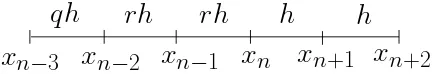
n+2Figure 1: 2-point 2-step method
In Fig 1, at each step, these methods will estimate the solution at two points with step size h concurrently using three back approximated values of the previous block with setp size rh. The methods are based on predictor-corrector scheme P E(CE)m of Adams type methods with variable step size.
Majid et al. [5] introduced the 2-point fully implicit block method (2PF). The value of yn+1 and yn+2 were approximated by integrating (1) over the
interval [xn, xn+1] and [xn, xn+2] respectively. In this paper, we try to derive
three possible type of 2-point 2-step methods (2PG, M2PG, M2PF), us-ing Lagrange interpolation polynomial. Durus-ing the implementation of 2PG method, the iteration Gauss Siedel style will be involved i.e. for obtaining corrector formula, the closest point in the interval for integrating (1) is con-sidered. Therefore the approximated values of yn+1 and yn+2 are obtained by
integrating (1), over the interval [xn, xn+1] and [xn+1, xn+2] respectively.
In M2PG method (modified 2PG method), our aim is to decrease the number of function called without losing desired accuracy. This may be done by involving the first approximated point, in the set of interpolation points for obtaining predictor formula for second point. Similar way can be applied for modifying 2PF method [5] and obtainingM2PF.
2
The 2PG method
In Figure 1, the solution of yn+1 andyn+2 at the points xn+1 and xn+2
respec-tively with step size h, will be approximated simultaneously using three back values at the points xn,xn−1,xn−2 of the previous two step with step size rh.
The method will compute two points concurrently using two earlier steps. The formula of the 2PGmethod are derived using Lagrange interpolation polynomial. The involved interpolation points for obtaining the corrector for-mula to approximate the solutions for the first and second point i.e. xn+1 and xn+2 are {(xn−2, fn−2), . . . , (xn+2, fn+2)}. The interval of integration for the
first and second point are [xn, xn+1], [xn+1, xn+2] respectively. by integrating
The 1st point,
The predictor formula are derived similarly, but the involved interpolation points are {(xn−3, fn−3), . . ., (xn, fn)}, so the predictor formula for first and
second point in terms of r and q are respectively,
The 1st point,
follow,
The remainder of the formula are the same as the 2PG method.
2.2
The M2PF method
The idea for deriving this method, is exactly the same idea for derivingM2PG method. Predictor formula for second point will stands for predicted value of first point. Therefore the predictor formula for second point is as follow,
yn+2=yn+h
The remainder of the formula are the same as the 2PF method.
3
stepsize control
The step size strategy in the code is the same as in [5], the choice for next step size will be limited to half, double or the same as the current step size. If the approximated solution at stepk, has desired accuracy, i.e. it is acceptable, therefore the choice for next step will be double or the same as current step size which may be specified by step size controller. Otherwise the step size controller will allow the step size to become half.
point, and the same corrector formula for that point of order p−1. The first predicted step size for hn+1 is given by,
hn+1 =τ ×hn×
T OL LT E
1p
where τ is a safety factor. The aim of utilizing this safety factor is to reduce the risk of the failure step. In the developed code, when the next step size is double, the ratio r is 0.5 and q can be 0.5 or 0.25, but if the next step size remain constant, r is 1 Andq can be 1 or 2 or 0.5. In case of step size failure, r is 2, and q is 2. In order to reducing cost of time, all the coefficients of the formula are stored in the developed code.
4
Absolute Stability
Here we will discuss the absolute stability of 2PGmethod using a linear first order test problem
y′
=f =λy (8)
The stability region is plotted when the step size ratio is constant, doubled and halved for the method. The test equation (8) is substituted into the corrector formula of the 2PGmethod. Setting the determinant of the corrector formula written in matrix form to zero will give the stability polynomial. The stability polynomials of 2PG method atr = 1,0.5,2 are as follow,
where ¯h=hλ and the stability regions are plotted in Figure 2.
r= 2
r= 1
r= 0.5
Figure 2: Stability region for 2PG method at r=2, 1 and 0.5
5
Numerical Results
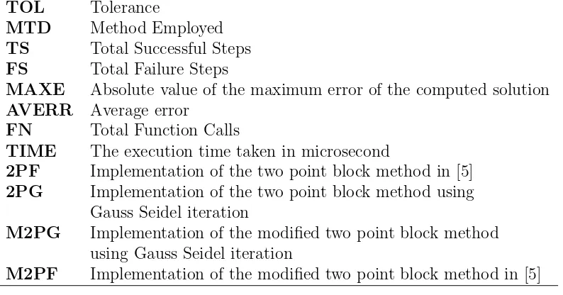
In order to show the efficiency and applicability of our presented methods, we consider four given problems to compare our computed solutions with the solutions obtained by method in [5]. The following notation are used in the tables:
TOL Tolerance
MTD Method Employed TS Total Successful Steps FS Total Failure Steps
MAXE Absolute value of the maximum error of the computed solution AVERR Average error
FN Total Function Calls
TIME The execution time taken in microsecond
2PF Implementation of the two point block method in [5] 2PG Implementation of the two point block method using
Gauss Seidel iteration
M2PG Implementation of the modified two point block method using Gauss Seidel iteration
M2PF Implementation of the modified two point block method in [5]
Problem 1: y′ =
−0.5y, y(0) = 1, [0,20] Exact solution: y(x) =e−0.5x
Source: Artificial problem
Problem 2: Nonlinear non stiff Krogh’s problem y′
β1 =β2 = 0.2, β3 = 0.3, β4 = 0.4
Exact solution: yi(x) = 1+cieβiβix, ci =−(1 +βi)
Source: Johnson and Barney [4]
Problem 3: A two-body orbit problem (Mildly stiff) y′
Problem 4: Linear nonstiff complex eigenvalues y′
Source: Johnson and Barney [4] The error calculated are defined as
(ei)t=
corresponds to the absolute error test, A = 0, B = 1 corresponds to the relative error test and finally A = 1, B = 1 corresponds to the mixed error test. The mixed error test is used for all the above problems. The maximum error and average error are defined as follows:
M AXE= max
Where N is the number of equation in the system, T S is the number of suc-cessful steps andP is the number of points in the block. In the code, we iterate the corrector to convergence using the convergence criteria:
yn+2r+1 −yrn+2
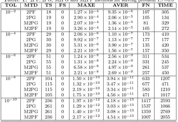
Table 1: 2PF, 2PG, M2PG and M2PF methods for solving problem 1,τ=0.8
TOL MTD TS FS MAXE AVER FN TIME
10−2 2PF 18 0 1.27×10⁻⁴ 9.35×10⁻⁶ 107 305
2PG 19 0 2.90×10⁻⁴ 2.06×10⁻⁵ 105 134
M2PG 19 0 2.07×10⁻⁴ 1.36×10⁻⁵ 81 329
M2PF 19 0 3.26×10⁻⁴ 2.14×10⁻⁵ 105 272
10−4 2PF 29 0 2.06×10⁻⁶ 1.10×10⁻⁷ 173 410
2PG 30 0 9.92×10⁻⁷ 1.13×10⁻⁷ 177 177
M2PG 30 0 5.31×10⁻⁶ 3.90×10⁻⁷ 135 420
M2PF 29 0 2.21×10⁻⁶ 1.56×10⁻⁷ 157 350
10−6 2PF 51 0 1.24×10⁻⁸ 2.56×10⁻⁹ 311 534
2PG 55 0 1.31×10⁻⁸ 2.24×10⁻⁹ 331 245
M2PG 55 0 6.58×10⁻⁸ 4.97×10⁻⁹ 261 537
M2PF 51 0 2.21×10⁻⁸ 2.69×10⁻⁹ 257 450
10−8 2PF 104 0 1.50×10⁻¹⁰ 3.94×10⁻¹¹ 633 1207
2PG 115 0 1.32×10⁻¹⁰ 3.47×10⁻¹¹ 677 471
M2PG 115 0 2.19×10⁻¹⁰ 3.34×10⁻¹¹ 583 1210
M2PF 105 0 1.75×10⁻¹⁰ 4.56×10⁻¹¹ 471 1017
10−10 2PF 236 0 1.97×10⁻¹² 4.18×10⁻¹³ 1417 2593
2PG 261 0 1.29×10⁻¹² 3.03×10⁻¹³ 1537 1066
M2PG 261 0 1.40×10⁻¹² 3.08×10⁻¹³ 1359 2769
M2PF 236 0 2.17×10⁻¹² 4.54×10⁻¹³ 1007 2055
Table 2: 2PF, 2PG, M2PG and M2PF methods for solving problem 2,τ=0.8
TOL MTD TS FS MAXE AVER FN TIME
10−2 2PF 20 0 3.02×10⁻⁴ 6.19×10⁻⁵ 121 864
2PG 22 0 3.76×10⁻⁴ 9.16×10⁻⁵ 127 569
M2PG 22 0 1.58×10⁻⁴ 4.45×10⁻⁵ 97 813
M2PF 20 0 4.94×10⁻⁴ 5.25×10⁻⁵ 115 778
10−4 2PF 34 0 2.12×10⁻⁶ 1.382×10⁻⁶ 217 918
2PG 39 0 1.74×10⁻⁶ 1.00×10⁻⁶ 229 620
M2PG 39 0 3.19×10⁻⁶ 2.04×10⁻⁶ 169 870
M2PF 34 0 3.04×10⁻⁶ 1.21×10⁻⁶ 181 848
10−6 2PF 66 0 2.81×10⁻⁸ 2.49×10⁻⁸ 419 1588
2PG 76 0 1.87×10⁻⁸ 1.48×10⁻⁸ 449 1206
M2PG 76 0 2.84×10⁻⁸ 1.05×10⁻⁸ 353 1554
M2PF 66 0 2.81×10⁻⁸ 2.40×10⁻⁸ 325 1396
10−8 2PF 143 0 3.47×10⁻¹⁰ 3.43×10⁻¹⁰ 875 3669
2PG 167 0 1.70×10⁻¹⁰ 1.66×10⁻¹⁰ 987 2626
M2PG 167 0 1.42×10⁻¹⁰ 6.93×10⁻¹¹ 815 3725
M2PF 143 0 3.44×10⁻¹⁰ 3.39×10⁻¹⁰ 659 3177
10−10 2PF 331 0 3.46×10⁻¹² 3.80×10⁻¹² 1985 7512
2PG 394 0 1.46×10⁻¹² 1.60×10⁻¹² 2335 6150
M2PG 394 0 1.25×10⁻¹² 6.76×10⁻¹³ 1949 8183
M2PF 331 0 3.73×10⁻¹² 3.96×10⁻¹² 1413 6546
Table 3: 2PF, 2PG, M2PG and M2PF methods for solving problem 3,τ=0.8
TOL MTD TS FS MAXE AVER FN TIME
10−2 2PF 30 0 1.02×10⁻¹ 2.23×10⁻² 261 1512
2PG 30 0 6.99×10⁻² 1.64×10⁻² 273 1081
M2PG 30 0 2.16×10⁻¹ 5.04×10⁻² 229 1306
M2PF 30 0 8.26×10⁻² 2.22×10⁻² 247 1498
10−4 2PF 61 0 1.47×10⁻³ 3.87×10⁻⁴ 443 2029
2PG 61 0 1.45×10⁻³ 3.79×10⁻⁴ 453 1560
M2PG 61 0 1.64×10⁻³ 4.32×10⁻⁴ 439 1858
M2PF 61 0 1.70×10⁻³ 4.47×10⁻⁴ 415 1959
10−6 2PF 137 0 2.01×10⁻⁵ 6.01×10⁻⁶ 1039 4681
2PG 139 0 1.92×10⁻⁵ 5.59×10⁻⁶ 1047 3620
M2PG 139 0 1.78×10⁻⁵ 4.89×10⁻⁶ 801 3714
M2PF 137 0 1.87×10⁻⁵ 5.57×10⁻⁶ 795 4006
10−8 2PF 322 0 2.09×10⁻⁷ 6.36×10⁻⁸ 1907 9825
2PG 327 0 1.96×10⁻⁷ 5.68×10⁻⁸ 1937 7076
M2PG 327 0 1.95×10⁻⁷ 5.73×10⁻⁸ 1913 8965
M2PF 322 0 1.80×10⁻⁷ 5.23×10⁻⁸ 1295 8249
10−10 2PF 781 0 2.21×10⁻⁹ 6.99×10⁻¹⁰ 4657 23027
2PG 797 0 2.09×10⁻⁹ 6.33×10⁻¹⁰ 4753 17455
M2PG 797 0 2.05×10⁻⁹ 6.19×10⁻¹⁰ 4687 21766
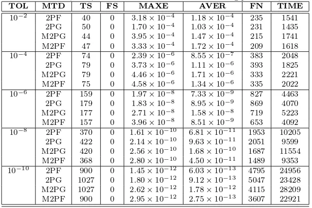
Table 4: 2PF, 2PG, M2PG and M2PF methods for solving problem 4,τ=0.5
TOL MTD TS FS MAXE AVER FN TIME
10−2 2PF 40 0 3.18×10⁻⁴ 1.18×10⁻⁴ 235 1541
2PG 50 0 1.70×10⁻⁴ 1.03×10⁻⁴ 231 1435
M2PG 44 0 3.95×10⁻⁴ 1.47×10⁻⁴ 215 1741
M2PF 47 0 3.33×10⁻⁴ 1.72×10⁻⁴ 209 1618
10−4 2PF 74 0 2.39×10⁻⁶ 8.55×10⁻⁷ 383 2048
2PG 79 0 3.73×10⁻⁶ 1.11×10⁻⁶ 393 1825
M2PG 79 0 4.46×10⁻⁶ 1.71×10⁻⁶ 333 2221
M2PF 75 0 4.58×10⁻⁶ 1.34×10⁻⁶ 335 2022
10−6 2PF 159 0 1.97×10⁻⁸ 7.33×10⁻⁹ 827 4463
2PG 179 0 1.83×10⁻⁸ 8.95×10⁻⁹ 869 4070
M2PG 177 0 2.71×10⁻⁸ 1.58×10⁻⁸ 719 5223
M2PF 157 0 3.96×10⁻⁸ 8.51×10⁻⁹ 653 4092
10−8 2PF 370 0 1.61×10⁻¹⁰ 6.81×10⁻¹¹ 1953 10205
2PG 422 0 2.14×10⁻¹⁰ 9.63×10⁻¹¹ 2051 9599
M2PG 420 0 2.56×10⁻¹⁰ 1.68×10⁻¹⁰ 1687 11554
M2PF 368 0 2.80×10⁻¹⁰ 4.50×10⁻¹¹ 1489 9353
10−10 2PF 900 0 1.45×10⁻¹² 6.03×10⁻¹³ 4795 24956
2PG 1027 0 1.80×10⁻¹² 9.12×10⁻¹³ 5047 23428
M2PG 1027 0 2.62×10⁻¹² 1.78×10⁻¹² 4115 28209
M2PF 900 0 2.95×10⁻¹² 2.75×10⁻¹³ 3607 22921
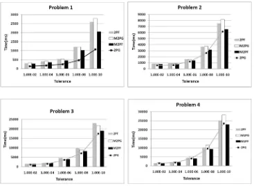
Figure 4: Results of execution time for Problem 1-4
From Tables (1-4), it can be observed that in all tested problems, the total number of steps and the maximum errors obtained by M2PF and M2PG meth-ods, are comparable to those, obtained by 2PF and 2PG methods respectively. However, in Fig 3, it is obvious that, the number of function called taken by M2PF is less than that in other methods, specially for finer tolerance. This could be justified by the fact that, M2PF method needs less iteration for the solution to be convergent. Since in M2PF the order of predictor formula for second point is greater than that in 2PF and 2PG, so the convergence crite-ria will be satisfied and M2PF doesn’t need more iterations. Also in M2PF method the value of yn which has obtained its sufficient accuracy in previous
block is involved for obtaining the predicted value for the second point in the current block. But in M2PG method the value of yn+1 which is in current block and it has not obtained its desired accuracy is involved. Therefore, the M2PG method needs more iterations.
called between M2PF and 2PG methods (especially for finer tolerance).
6
Conclusion
In this paper, we proposed three methods (2PG, M2PG, M2PF) for solving system of initial value problems (ODEs). After comparing the results of these methods with 2PF method [5] and with them selves as well, we can conclude that, each of these methods will give comparable results in terms of maximum error and total number of steps. But M2PF method has less number of function called compare to other methods, whereas the execution time of 2PG method is faster than the other methods.
References
[1] K. Burrage, Efficient Block Predictor-Corrector Methods with a Small
Number of Corrections, J. of Comp. and App. Math., 45 (1993), 139-150.
[2] Fatunla, Block Methods for Second Order ODEs, Intern. J. Comp. Math. 41(1990), 55-63.
[3] E. Hairer, S.P. Norsett, G. Wanner, Solving Ordinary Differential Equa-tions I, Springer-Verlag, Berlin, 1993.
[4] A.I. Johnson,J.R. Barney, Numerical solution of large systems of stiff or-dinary differential equations, in:L. Lapidus,W.E. Schiesser(Eds.), Modu-lar Simulation Framework, Numerical Methods for Differential Systems, Academic Press Inc, New York, 1976,pp.97-124.
[5] Z.A. Majid, M. Suleiman, F. Ismail, M. Othman 2-point 1 block Diago-nally and 2-point 1 block Fully Implicit Methods for solving First Order Ordinary Differential Equations, Proceedings of the 12th National
Sym-posium on Mathematical Sciences, No 34.
[6] W.E. Milne, Numerical Solution of Differential Equations, Wiley, New York, 1953.
[7] J.B. Rosser,A Runge-Kutta for all seasons, SIAM Rev. 9 (1967), 417-452.
[8] L.F. Shampine and H. A. Watts, Block implicit one-step methods, Math. comp. 23(1969),731-740 (1991)243-254.