DOI 10.1007/s10569-006-9010-4 O R I G I NA L A RT I C L E
The scattering map in the planar restricted three body
problem
E. Canalias · A. Delshams ·J. J. Masdemont · P. Roldán
Received: 15 November 2005 /Accepted: 31 January 2006 / Published online: 15 August 2006
© Springer Science+Business Media B.V. 2006
Abstract We study homoclinic transport to Lyapunov orbits around a collinear libration point in the planar restricted three body problem. A method to compute homoclinic orbits is first described. Then we introduce the scattering map for this problem (defined on a suitable normally hyperbolic invariant manifold) and we show how to compute it using the informa-tion already obtained for the homoclinic orbits. An example applicainforma-tion to Astrodynamics is also proposed.
Keywords Restricted three body problem·Homoclinic orbits·Normally hyperbolic invariant manifolds·Scattering map
1 Introduction
Interest in the dynamics around the Lagrangian points has been increasing in the last decades, asL1andL2of the Sun–Earth and Earth–Moon systems have been selected for a wide variety of spatial missions (see Farquhar 1972; Breakwell et al. 1974; Gómez et al. 1991; Canalias and Masdement 2005). The introduction of invariant manifolds as a means to describe the phase space around these points yields not only a more efficient determination of the desired transfers but also an adaptable procedure for mission analysis. Invariant manifolds dominate the dynamics and mass transport in the studied system and in the whole Solar System. In this context, homoclinic trajectories provide zero cost transfers from a libration orbit aroundLi
(i=1,2) to another one. In the planar case, there is only one periodic motion aroundL1. In particular, homoclinic trajectories are not a means to go from one orbit to another one, but to leave the periodic orbit at a certain point and approach it again in a different point. This feature has possible astrodynamical applications, such as the placement of different satellites in previously chosen points of the same orbit.
E. Canalias·A. Delshams·J. J. Masdemont·P. Roldán (
B
) Departament de Matemàtica Aplicada I,This paper includes a detailed explanation of the numerical method used for finding ho-moclinic connections by intersecting the stable and unstable manifold of planar Lyapunov orbits aroundL1, which was presented for the first time in Canalias and Masdemont (2006). Further, we look at the set of Lyapunov orbits around a collinear libration point as a nor-mally hyperbolic invariant manifold, with associated stable and unstable invariant man-ifoldsWs,Wu. These manifolds are important because they organize the dynamics of the system. The hyperbolic invariant manifoldsWs,Wu intersect transversally along families of homoclinic orbitsHj,i.
Following Delshams et al. (2000b, 2006), we define the scattering map Sj,i: →
associated to a family of homoclinic orbits. The scattering map relates two trajectories in
through a homoclinic orbit in the familyHj,i.
Exploiting the fact that there is only one Lyapunov orbit around the libration point for each value of the Jacobi constant, we show that the scattering map for the planar restricted three body problem (PRTBP) has a simple form. Specifically, it is an integrable twist map.
Using only three points from each homoclinic orbit in the family Hj,i, we are able to compute the associated scattering map. For illustration purposes, in this paper we compute the scattering map for several families of homoclinic orbits to theL1libration point in the Earth–Moon model.
Our future goal is to give a complete description of homoclinic and heteroclinic phenom-ena in the spatial restricted three body problem (RTBP). This paper is a first step toward that goal, where we have used the PRTBP as a test case for the concepts and methods involved.
2 Methodology
The RTBP is a model of the motion of an infinitesimal particle, affected by the gravitational attraction of two massive bodies (primaries), which describe circular orbits around their com-mon center of masses. When the movement of the massless particle is only studied in the plane of motion of the primaries, the problem becomes planar (PRTBP).
Taking adequate units of mass, length and time we can simplify the equations of motion. Furthermore, the following synodical system of reference is taken: the origin set at the center of masses of the two primaries, theX-axis given by the line that goes from the smallest to the biggest primary (with this orientation) and theY-axis taken so thatXYis a planar positively oriented coordinate system. In our synodical system the primary of massµ(small) is always located at (µ−1,0) and the primary of mass 1−µat (µ,0) (Szebehely 1967). The equations
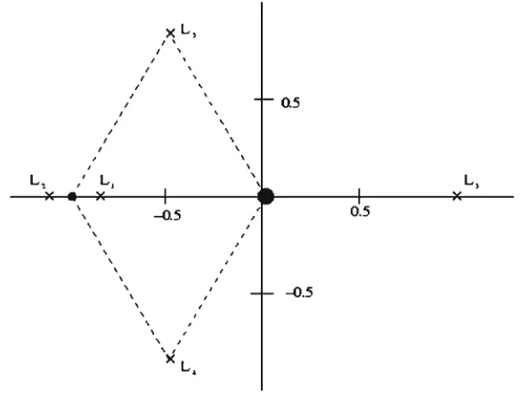
Fig. 1 The five equilibrium points of the RTBP
points) are found as the third vertex of the two equilateral triangles that can be formed using the primaries as vertices (Fig. 1).
Introducing momentapx = ˙x−yandpy= ˙y+x, the PRTBP equations of motion cast
into a Hamiltonian system. The Hamiltonian function is
H(x,y,px,Py)= 1
2(p 2
x+p2y)+ypx−x py−
1−µ r1
− µ
r2
−1
2µ(1−µ)
We define the Jacobi constant,C,
C(x,y,x,˙ y)˙ = −(x˙2+ ˙y2)+2(x,y) (2)
withas in (1). It is easily proved thatC = −2H. Consequently, the Jacobi constant is a first integral of the RTBP.
In this work, we will focus on the dynamics around the equilibrium pointL1. The linear behavior of this point is of the type center×saddle. The hyperbolicity introduced by the sad-dle component is inherited by all the orbits in a large vicinity ofL1. Moreover, it is responsible for the existence of unstable and stable manifolds arising from the aforementioned orbits.
2.1 Planar Lyapunov orbits
For each value of the Jacobi constant, there is a unique planar Lyapunov orbit homeomorphic toS1aroundL1. This is the unique periodic motion around theL1for the planar case, and the one we use in this work.
Planar Lyapunov orbits and their hyperbolic manifolds can be computed using Lindstedt–Poincare procedures. In this way one obtains their expansions in convenient RTBP´
coordinates.
¨¯
depend only onµand the selected equilibrium point (see Masdemont 2005). We note that in (3) the linear terms appear in the left hand side part of the equations and the nonlinear ones on the right-hand side. The solution of the linear part of Eq. (3) is:
¯
Theαs are free amplitudes.α1andα2are the ones associated with the hyperbolic man-ifolds. Ifα1 = α2 = 0, we have the linear part of the Lyapunov orbit with amplitudeα3. Whenα1 =0 andα2 =0 we have orbits tending exponentially fast to the Lyapunov orbit of amplitudeα3when time tends to infinity (stable manifold). On the contrary whenα2=0 andα1 = 0, orbits leave the vicinity of the Lyapunov exponentially fast in forward time (unstable manifold).
When we consider also the nonlinear terms of (3), solutions close toL1are obtained by means of formal series in powers of the amplitudes of the form:
¯
zero. It is important to note that for the frequency series, the coefficientωi j k =0 only if i = j. Thus, we can write,
ω=ωlk(α1α2)lαk3, λ=
λlk(α1α2)lαk3. (6)
In the computations, the series are truncated at a certain (high) order (Masdemont 2005). Nevertheless, we note that the meaning of the amplitudes in the nonlinear expansions (5) is the same one as in the linear solutions (4).
Therefore, in these coordinates, we can write the Lyapunov orbit of amplitudeαas,
λα= {X =(α1, α2, α3, φ)∈R3×T: α1=α2=0, α3=α, φ∈T}.
Notice that in the PRTBP there is a bijective correspondence between values of the Jacobi constant and values of the amplitude α3. Thus, we can also consider coordinates X =(α1, α2,C, φ)∈R3×Tand write the above Lyapunov orbit as
λC = {X=(α1, α2,C, φ)∈R3×T:α1=α2=0,C=C, φ∈T},
We can now define the local unstable and stable manifolds associated toλC:
WλsC,loc = {(0, α2,C, φ): α2∈I2 ⊂R, φ∈T}, Wλu
C,loc = {(α1,0,C, φ): α1∈I1⊂R, φ∈T},
whereI1×I2⊂R2is an open rectangle containing the origin.
2.2 Hyperbolic manifolds
In the previous section, we saw how the Lyapunov orbits and their stable and unstable manifolds can be described semi-analytically up to a certain order. Nevertheless, as far as manifolds are concerned, the analytical description is used only in a small vicinity of the Lyapunov orbit. For the rest of the tube, the manifold is obtained by numerically integrating this semi-analytical expression.
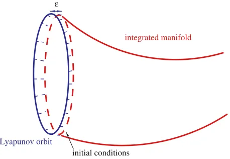
That is, there are two different parts in the description of each manifold. By settingα1= ±ǫ andα2=0 (respectively,α2 = ±ǫandα1 =0), and the rest of the amplitudes and phases fixed to the chosen Lyapunov orbit values, a point on the local unstable (respectively, stable) invariant manifold is obtained in the series (5). Sett = 0, so we can refer to these points asinitial conditions. Furthermore, the aforementioned initial conditions are at a distance of orderǫfrom the Lyapunov orbit. The part of the local manifold which asymptotically joins them with the Lyapunov orbit is described analytically by the same series for values of time
t=0. In the caseα1=0, negative values of time tending to−∞result in points belonging to the local unstable manifold and approaching the Lyapunov orbit exponentially fast (respec-tively, positive times tending to+∞forα1=0). This part is represented, schematically, in Fig. 2 as the small gap between the ‘Lyapunov orbit’ and the ‘initial conditions’.
For other values of time (positive for the unstable case and negative for the stable), the manifold tubes can be continued by integrating the initial conditions: in forward time for the caseα1 =0 and backward in time forα2 =0 (part labelled as ‘integrated manifold’ in Fig. 2). Note that this numerical integration is necessary, as it provides us with an accu-rate description of the manifolds in regions where the Lindstedt–Poincaré expansions are no longer valid due to the large distance to the equilibrium point.
Lyapunov orbit
initial conditions
integrated manifold
ε
2.3 Numerical computation of homoclinic trajectories
In order to look for homoclinic orbits of a Lyapunov orbit emerging from L1, we will use a Poincaré section. This is a common technique in the study of dynamical systems, and consists of observing the flow of the system only in the points that cross a given section. In this way, the flow is studied in a lower dimensional space, but relevant information can still be derived. The stable and unstable manifolds of Lyapunov planar orbits are two-dimensional objects (see Sect. 2.2). If we study them only in their cut with a Poincaré section (i.e.= {(x,y,x˙,y):˙ x=K}, whereK is a constant), the resulting objects are closed curves, and therefore, much easier to study and represent. These two closed curves may intersect transversally in several points. Each intersection point belongs to a different homoclinic connection to the Lyapunov orbit.
One can consider the first, second, and so on, cut of the invariant manifolds with the Poincaré section, and obtain in this way different closed curves which may have a different number of intersections and therefore, a different number of homoclinic connections (which perform several loops around the primary).
So, takeas the plane in the state space of the points withx= −1+µ. Now, the process of finding homoclinic connections,γC, to a Lyapunov orbit,λC, consists of three parts:
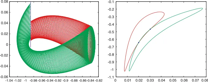
1. Integration of the manifolds(WλsC,WλuC)arising from the Lyapunov orbits(λC)until
they cut the Poincaré section(see Fig. 3).
2. Detection of intersections between the cuts of the asymptotic manifolds (WλsC ∩and
WλuC ∩) in the Poincaré section (see Fig. 3).
3. Refinement of the intersections up to a certain precision.
2.3.1 Integration of the manifolds
As it has been said, when the value ofCis chosen,α3is fixed. In order to take initial conditions on the unstable (respectively, stable) local manifolds in (5) we setα1 = ±ǫ (respectively, α2 = ±ǫ).ǫis a small parameter(≈10−3), and the sign indicates toward which branch of the manifold we will integrate: In L1,+ǫmeans toward the small primary, while−ǫmeans toward the interior region.
-1.04 -1.02 -1 -0.98 -0.96 -0.94 -0.92 -0.9 -0.88 -0.86-0.84 -0.82 -1.1
The discretization on the initial conditions arises from takingnphases around the Lyapunov orbitλC,θ1i(0)=φi =2πi/n, i=0, . . . ,n−1.
The bunch of orbits launched by these kind of initial conditions, with the series in (5) truncated at order 15, form manifold tubes. A Runge–Kutta–Fehlberg method of orders 7–8 is then used for the integration. Note that order 15 provides a precise approximation to the manifolds which is adequate to fulfil very stringent numerical requirements (in particular, enough for the purposes of this work).
As the equation of the Poincaré section is x = µ−1, the number of cuts (N) with the section can be easily controlled by studying the sign ofx(t)+1−µ. WhenNmatches the desired number of cuts, a one-dimensional Newton procedure is used in order to obtain the point on the section with an accuracy of at least 10−12(i.e.|x(t)+1−µ|<10−12).
2.4 Detection of intersections between the cuts of asymptotic manifolds in the Poincaré section
Once the integration is completed, we have a set of points on the Poincaré section belonging to a discrete bunch of trajectories lying on the manifolds (ntrajectories ifnphases where used). So, the result of joining these points is a polygon made ofnsegments. The integration is performed for both the unstable manifold and the stable one, so two curves are obtained on the Poincaré section (see the right picture in Fig. 3).
The next step that has to be taken is to check for intersections on the sectionbetween each segment of one of the curves and all the segments of the other curve. All in all,(n1)×(n2)≈ O(n2)(ninumber ofθ1in manifoldi) comparisons between segments. This is why it is not worth taking largenvalues, because it does not enhance the precision of the final cut, but increases the computational effort. Nevertheless,nhas to be large enough for the cuts on the Poincaré section to be well determined with an approximatedS1structure when the segments are joined together (for instance,n1=n2=100).
There is a correspondence between each segment(a,b)on the section and a segment
(φa, φb)∈T, such thata(respectivelyb) is the integrated point corresponding to the initial condition on the manifold withθ1=φa(respectivelyφb) Therefore, at the end of this pro-cess we store four phase values for each detected cut. Two of them for the unstable manifold,
(φau, φub)and the other two(φsa, φbs)for the stable manifold.
2.4.1 Refinement of the intersections
We start with the intervals found in the previous step, and we look forφu ∈ [φau, φub]and φs ∈ [φas, φsb], which define the exact initial conditions of the connecting trajectory.
We use a secant-like method to find the intersection between the segmentssu0=(φa0 u , φbu0)
andss0 =(φa0
s , φsb0), which we know have a nonempty intersection ifa0 =aandb0 =b. The pair of intersecting phases divides each of the original segments in two, so four new segments are defined. Now, we look for intersections between the segments associated with
WλuC and the ones associated withWλsC. Only one of the four checks should be positive. So, we store only the four phases which are in the border of the new intersecting segmentssu1
andss1. Thus, we have again[φa1
u , φbu1],[φsa1, φsb1], but the longitude of the intervals has been
reduced.
We iterate the processktimes until|sk
u| + |sks| = |φ ak
When the three steps have been successfully carried out for an appropriateC, we have
(φu, φs), the phases on the Lyapunov orbit defining the connection. We have the intersecting
point on the Poincaré section, and the corresponding integration times as well.
So, the connecting trajectory can be reconstructed by taking the following initial conditions:
• For the unstable manifold:(α1, α2, α3, θ1)=(10−3,0, α3(C), φu). • For the stable manifold:(α1, α2, α3, θ1)=(0,−10−3, α3(C), φs)
The integration of these initial conditions yields the connection. Obviously, the one on the unstable manifold has to be integrated forward in time, while the other one backward.
Once a homoclinic connection to a Lyapunov orbitλC has been found, some other
con-necting trajectories can be found to nearby Lyapunov orbitsλC′, by slightly varying the initial conditions (due to the analytic continuous dependence of the solutions of the dynamical equa-tions w.r.t. these initial condiequa-tions). A group of trajectories which are coincident in some of the initial parameters giving rise to one-parameter family of homoclinic trajectories will be called a family of homoclinic trajectories and denoted by H. We can classify the families of homoclinic trajectories to L1planar Lyapunov orbits depending on the number of cuts with the Poincaré section or equivalently, the number of loops, j, around the small primary that the trajectories do. In addition, for the same number of cuts with the section, more than one family is obtained. In particular, the number of families is equal to the number of intersections between the manifolds on the section.
To construct these continuous one-parameter families Hj,i of homoclinic trajectories, we consider only those intervals(Cj,i
− ,C
j,i
+ )of Jacobi constants for which the intersections
between the manifolds are transversal. The specific valuesC±j,iare candidates to bifurcation homoclinic intersections. number of loops andi is the integer identifying the family depending on theycoordinate on the Poincaré section (i =1 corresponding to the families yielding the intersection with smallesty).
Notice that, by construction, for anyjandi, and anyC∈(C−j,i,C+j,i)there exists a unique homoclinic orbitγCj,i ⊂Hj,ito the Lyapunov orbitλC.
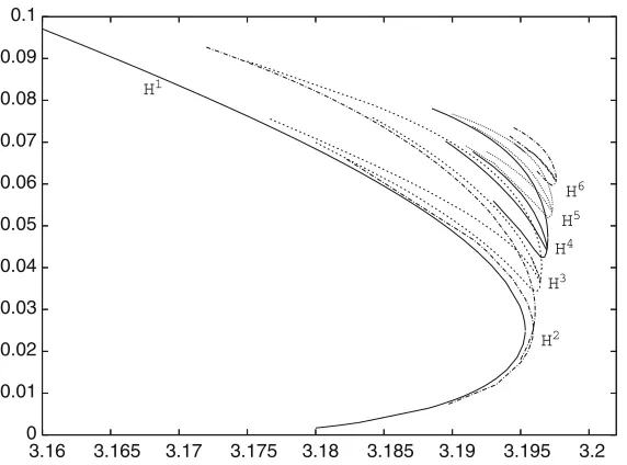
Figure 4 is a representation of the families that have been obtained using the procedure explained above for the Earth–Moon mass parameterµ. The notation is simplified in the figure toHj. Each one of the branches corresponds toHj,iwithiincreasing upwards. The
x-axis in the figures corresponds to the value of the Jacobi constant, and they-axis to the
y-coordinate of the trajectory in one of the cuts with the Poincaré section in adimensional RTBP coordinates.
0 0.01 0.02 0.03 0.04 0.05 0.06 0.07 0.08 0.09 0.1
3.16 3.165 3.17 3.175 3.18 3.185 3.19 3.195 3.2
Fig. 4 Families ofL1homoclinic orbits in the Earth–Moon case. On thehorizontal axis, value of the Jacobi constant, and on thevertical axis,ycoordinate of the connecting orbit on the Poincaré section
3 Scattering map
3.1 The NHIMand associated hyperbolic manifolds
In Sect. 2.1, Lindstedt–Poincaré variables for the restricted three body problem around the fixed point have been introduced. A point in phase space close to L1is written in these vari-ables asX =(α1, α2, α3, φ)∈B×R×T, whereB= I1×I2 ⊂R2is an open rectangle containing the origin inR2.
These variables are convenient because they parametrize the invariant manifolds present in the system in a natural way.
Let[C1,C2]be an interval of energy values such that∀C ∈ [C1,C2]there exists (at least) one orbit homoclinic toλC. Following Delshams et al. (2006), we introduce the set
= {X∈B×R×T:α1=α2=0,C∈ [C1,C2]} (8)
=
C∈[C1,C2]
λC. (9)
This set is a two-dimensional manifold with boundary. It is invariant for the flowtof the
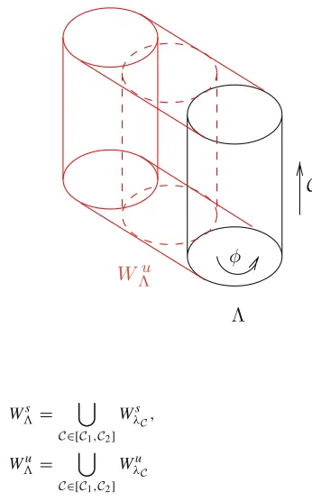
system. The manifoldis topologically[C1,C2] ∈T. A point in the manifold is parametrized by(C, φ).is a subset of the so-called center manifold (Fig. 5).
Fig. 5 Schematic representation of the normally hyperbolic invariant manifoldand one of its asymptotic manifoldsWu
The sets
Ws =
C∈[C1,C2]
WλsC,
Wu =
C∈[C1,C2]
WλuC
are called stable and unstable manifolds ofin normally hyperbolic theory. They are three-dimensional manifolds. A local parametrization is given by
W,s loc= {(0, α2,C, φ): α2∈I2⊂R,C∈ [C1,C2], φ∈T},
W,u loc= {(α1,0,C, φ): α1∈I1⊂R,C∈ [C1,C2], φ∈T}.
Recall the definition of the stable manifold of a pointXin a hyperbolic set:
WXs = {Y ∈R3×T: dist(t(X), t(Y))≤K(X)exp−λt, t→ ∞}. (10)
Notice the same timet int(X)andt(Y)and an exponent of convergenceλ > 0. In
general, this manifold isnotinvariant for the flow of the system. (It is the nonlinear analog of the contracting subspaceEs
xin the hyperbolic splitting of a hyperbolic invariant set. For an
introduction to hyperbolic invariant sets, see Robinson 1999). However, the stable manifold of a point satisfies the property
t(WXs)=Wst(X). (11)
In the case of the PRTBP, the local stable manifold of a point X+ =(0,0,C+, φ+)∈
is given by
WXs
+,loc= {(0, α2,C+, φ+): α2∈I2} (12) as one can easily check from Eqs. (5) and (6). Analogously, givenX−=(0,0,C−, φ−)∈,
WXu−,loc= {(α1,0,C−, φ−): α1∈I1}. (13)
It is thus evident that
W,s loc= X∈
WXs,loc and WXs,loc∩WYs,loc= ∅, ifX=Y
and by extension,
Ws =
X∈
WXs and WXs ∩WYs = ∅, ifX=Y. (14)
There is a similar foliation for the unstable manifold.
3.2 The dynamics in
In the case of the PRTBP, the dynamics restricted tois very simple. The normally hyper-bolic invariant manifold is foliated by invariant tori corresponding to periodic Lyapunov orbits. The flow onis given by
t(0,0,C0, φ0)=(0,0,C0, φ0+ωt), (15)
whereωis given in (6), and we will denote by
λt(C0, φ0)=(0,0,C0, φ0+ωt) (16)
the orbits in the torusλC0.
3.3 Definition of the scattering map
In this section, we are going to define a scattering mapSj,i for every familyHj,iof
homo-clinic orbits to. For ease of presentation, through this section we will drop the indices that identify a homoclinic family.
Consider a homoclinic familyHdefined on a given interval(C−,C+). Take a pointZ∗∈H
and letC∈(C−,C+)be its Jacobi constant, so thatZ∗∈γC. By definition of the stable and
unstable manifolds of(see (10)), there existX−∗,X+∗ ∈such that
dist(t(Z∗), t(X∗±))≤K(Z∗)exp−λ|t|, t→ ±∞,
which are unique by (14). Indeed, by preservation of the Jacobi constant,X∗−,X+∗ ∈λC.
Consider now an arbitrary point X−in the Lyapunov periodic orbit λC, so that X− =
τ(X−∗), withτ ∈ [0,TC), whereTC is the period ofλC. We defineX+=τ(X∗+)∈λC ⊂ , Z=τ(Z∗)∈γCand notice that
dist(t(Z), t(X±))≤K(Z)exp−λ|t|, t→ ±∞. (17)
The map
X−∈D⊂
S
−→X+∈D⊂, (18)
whereD= ∪C∈(C−,C+)λC, is called the scattering map and is characterized by the property
that
Notice that the scattering mapS=Sj,iand its domain of definitionD=Dj,idepend on the homoclinic familyHj,i.
Next we check this characterization. Assume that there existZ1,Z2∈HandX+,1,X+,2∈ with
dist(t(Zk), t(X−))≤K(Zk)exp−λ|t|, t→ −∞ (19)
but
dist(t(Zk), t(X+,k))≤K(Zk)exp−λ|t|, t→ +∞. (20)
SinceZ1,Z2 belong toγC, Z2 =t1(Z1), and imposing (19) and the fact thatλC is
peri-odic, one easily gets thatt1 =nTC for some integern. Imposing now (20), one finds that X+,1=X+,2. This proves that the scattering mapSis well defined and that it does not depend on the choice of the point Zin (17). Analogously, one can check thatS−1: X+ → X− is
also well defined.
An interesting property of the scattering map in the case of the planar restricted three body problem is that it commutes with the flow: for anyt ∈R
S(t(X−))=t(X+), (21)
which follows readily from the characterization (17) and the fact that if (17) holds for two pointsZ1andZ2thenZ2=t1(Z1)witht1=nTC.
We now look for the expression of the scattering map in the coordinates (C, φ) of
introduced in (8).
Due to the low dimensional nature of the PRTBP, one can easily describe the scattering map associated to a homoclinic manifold. LetX−,X+∈have Lindstedt–Poincaré variables
X− =(C, φ−),
X+ =(C, φ+),
so thatS(C, φ_+ωt)=(C, φ++ωt)by property (21). Introduce the phase shift
=(C)=φ+−φ−, (22)
which depends on the torus. Then we can express the scattering map as
S(C, φ)=(C, φ+(C)) (23)
for any(C, φ)∈(C_,C+)×T. Hence, the scattering map has the form of an integrable twist map. As a matter of fact, it is a nontrivial twist map, that is′(C)≡/0, as will be shown in the next section.
3.4 Computation of the scattering map
As explained in the previous section, the particular geometrical features of the PRTBP impose a strong structure for the scattering map associated to a homoclinic manifold. For every j,i,
• S=Sj,i can be computed independently on each torusλC ∈Dj,i.
• On a given torusλC, the scattering map is just a translationφ →φ+by a constant
shift=j,i(C).
Therefore, the problem of computingSreduces to computing(C)for any torus in the rangeC∈(Cj,i
− ,C
j,i
Remark 1 The characterization of the scattering map in terms of a scalar function(C)is
very specific of this problem, becauseCis a constant of motion and there is only one torus λCfor everyC. Obviously, this will not happen in the spatial RTBP, where theλChave to be
replaced by two-dimensional KAM invariant tori. ⊓⊔
Let us fixC∈(Cj,i
− ,C
j,i
+ )and consider the corresponding 1-torusλCand homoclinic orbit γC =γCj,i. We seekX−=(C, φ−)andX+=(C, φ+)inλC such that
Z∈WXu−
and
Z∈WXs+
for someZ∈γC.
Note thatX−andX+are related toZ asymptotically, so these two points cannot be found
fromZby direct iteration. The algorithm used in Sect. 2.3 to find the homoclinic connection
γC provides us withXu∈WλuC,Xs ∈WλsCandZ ∈γCrelated in the following way:
tu(Xu) =Z, ts(Xs) =Z.
The algorithm already givesXuandXsin Lindstedt–Poincaré coordinates
Xu =(α1, α2,C, φ)=(ǫ,0,C, φu),
Xs =(α1, α2,C, φ)=(0, ǫ,C, φs).
From (13),Xubelongs to the unstable manifold of the pointX˜−=(0,0,C, φu). Similarly, Xsbelongs to the stable manifold of the pointX˜+=(0,0,C, φs). By assertion (11),
Z =tu(Xu)∈Wu tu(X˜−),
Z =ts(Xs)∈Ws ts(X˜+). Thus the points we seek are
X− =tu(X˜−)=λtu(X˜−), X+ =ts(X˜+)=λts(X˜+).
In coordinates, they are given by
X− =(0,0,C, φ−)=(0,0,C, φu+tuω), X+ =(0,0,C, φ+)=(0,0,C, φs+tsω).
Therefore,
φ− =φu+tuω, φ+ =φs+tsω,
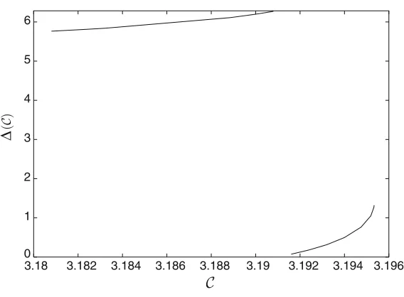
Fig. 6 Rotation angle associated toS1,1
3.5 Some numerical results
Using the method described in the previous section, we have computed the scattering maps associated to several homoclinic families in the PRTBP. The results presented here are for Lyapunov orbits aroundL1in the Earth–Moon model.
Recall from Sect. 3.3 that the scattering mapSj,iassociated to a given homoclinic family
Hj,iis characterized by a scalar functionj,i(C)defined on a domainC∈(C−j,i,C+j,i). The functionj,i(C)is the rotation angle that results from applyingSj,i to any point inλC.
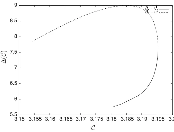
Consider the simplest homoclinic families H1,1andH1,2, which loop once around the small primary. Figures 6 and 7 show 1,1, respectively,1,2 in the same domains where the homoclinic families were computed (compare to Fig. 4). We also plot both functions together in Fig. 8 to show how they are a natural continuation of each other. In this way it is also easier to compare the intervals of Jacobi constants where j,i are defined. The functions are represented in the universal cover, instead of [0, 2π), to emphasize that each one is continuous.
Note that the slope of(C)goes to infinity at the bifurcation point. Note also that1,2(C) is a twist map for allC ∈ (C1−,2,C+1,2)except for a point where1,2 attains a maximum, giving rise there to a nontwist map (see Delshams and De la Llave 2000a).
3.6 Example application to astrodynamics
This section describes an example application of the scattering map to the design of space-craft trajectories in the restricted three body problem. The goal of this example is to illustrate the convenience and usefulness of the scattering map as a tool to study homoclinic and het-eroclinic phenomena in dynamical systems. Other applications can probably be found in the field of mission design or in a different field.
0 1 2 3 4 5 6
3.15 3.155 3.16 3.165 3.17 3.175 3.18 3.185 3.19 3.195 3.2
Fig. 7 Rotation angle associated toS1,2
5.5 6 6.5 7 7.5 8 8.5 9
3.15 3.155 3.16 3.165 3.17 3.175 3.18 3.185 3.19 3.195 3.2 ∆
∆
Fig. 8 Rotation functions associated toS1,1(solid line) andS1,2(dotted line)
Table 1 Rotation angle for several homoclinic families forC=3.19
1,1 1,2 2,3 2,4 3,1 3,2 3,3 3,4 4,1 4,2 4,4
6.197 2.615 2.529 5.767 2.437 5.611 5.662 2.702 5.594 2.578 5.876
The main drawback of this method is that the transfer times are longer than when using classical maneuvers.
In our example, let us fix some Lyapunov orbit for definiteness, sayλ=λCwithC=3.19.
There are several scattering mapsSHdefined onλ⊂, depending on the choice of
homo-clinic familyH. Recall from Sect. 3.3 thatλis parametrized by an angleφ, and the scattering map restricted toλis just a rigid rotation
φ→φ+.
Having computed several scattering maps numerically in Sect. 3.4, we know the values offor several homoclinic manifolds. Table 1 shows these values (in radians).
Each application of the scattering mapSHcorresponds to performing a homoclinic
excur-sion through a trajectoryγ ⊂H. In the example application, a homoclinic excursion consists in injecting a satellite into the unstable manifold of the Lyapunov orbit using station keeping like maintenance maneuvers, and then following the selected homoclinic trajectory, which naturally comes back to the Lyapunov orbit following its stable manifold. The result is that the satellite is shifted by an anglewith respect to its initial phase.
Therefore, the example problem can be formulated as follows: letIbe an index set that will be used to index the finite set of scattering maps (or rotation angles) shown in Table 1. Equiv-alently,Ialso indexes the homoclinic manifolds considered. Suppose thatxA=(C, φA)and
xB =(C, φB) ∈are the initial conditions of the two spaceships on the Lyapunov orbit.
Find a sequence(i1,i2, . . . ,in)∈In such that
dist(Sin◦ · · · ◦Si2◦Si1(x
A),xB) <d
or equivalently
dist(φA+i1+i2+ · · · +in, φB) <d,
wheredis a prescribed distance.
This would correspond tonhomoclinic excursions for spaceshipA. Obviously, one could apply the scattering map to bothφAandφB, i.e., applying maneuvers to both spaceships.
Acknowledgements This research has been supported by the MCyT-FEDER grant BFM2003-09504, and the Catalan grant 2003XT-00021. E.C. acknowledges the fellowship AP2002–1409 of the Spanish Govern-ment. The authors thank R. de la Llave for his insightful comments on the scattering map.
References
Breakwell, J.V., Kamel, A.A., Ratner, M.J.: Station-keeping for a translunar communication station. Celestial Mech.10, 357–373 (1974)
Canalias, E., Masdemont, J.J.: Lunar space station for providing services to solar libration point missions. In 56th International Astronautical Federation Congress, Fukuoka, Japan (2005)
Canalias, E., Masdemont, J.J.: Homoclinic and heteroclinic transfer trajectories between Lyapunov orbits in the Sun–Earth and Earth–Moon Systems. Discrete Contin. Dyn. Syst.14, 261–279 (2006)
Delshams, A., de la Llave, R., Seara, T.M.: A geometric approach to the existence of orbits with unbounded energy in generic periodic perturbations by a potential of generic geodesic flows ofT2. Comm. Math. Phys.209(2), 353–392 (2000b)
Delshams, A., de la Llave, R., Seara, T.M.: A geometric mechanism for diffusion in Hamiltonian systems overcoming the large gap problem: heuristics and rigorous verification on a model. Mem. Amer. Math. Soc.179(844), 1–141 (2006)
Farquhar, R.W.: A halo orbit lunar station. Astronautics and Aeronautics10(6), 52–63 (1972)
Gómez, G., Jorba, A., Masdemont, J.J., Simó, C.: A dynamical systems approach for the analysis of the SOHO mission. Third International Symposium on Spacecraft Flight Dynamics, ESA/ESOC, pp. 449– 454, (1991)
Masdemont, J.J.: High-order expansions of invariant manifolds of libration point orbits with applications to mission design. Dyn. Syst.20(1), 59–113 (2005)
Robinson, C.: Dynamical systems. Studies in Advanced Mathematics 2nd edn. Stability, symbolic dynamics and chaos, CRS Press, Boca Raton (1999)