Ideal Midline Detection Using Automated Processing of Brain CT Image

(1)

http://dx.doi.org/10.4236/ojmi.2013.32007 Published Online June 2013 (http://www.scirp.org/journal/ojmi)

Ideal Midline Detection Using Automated Processing

of Brain CT Image

Xuguang Qi1*, Ashwin Belle1, Sharad Shandilya1, Wenan Chen2, Charles Cockrell3, Yang Tang3, Kevin R. Ward4, Rosalyn H. Hargraves5, Kayvan Najarian1

1

Department of Computer Science, School of Engineering, Virginia Commonwealth University, Richmond, USA

2

Department of Biostatistics, School of Medicine, Virginia Commonwealth University, Richmond, USA

3

Department of Radiology, School of Medicine, Virginia Commonwealth University, Richmond, USA

4

Department of Emergency Medicine and Michigan Critical Injury and Illness Research Center, University of Michigan, Ann Arbor, USA

5

Department of Electrical and Computer Engineering, Virginia Commonwealth University, Richmond, USA Email: *qix2@vcu.edu

Received April 2, 2013; revised May 7, 2013; accepted May 21, 2013

Copyright © 2013 Xuguang Qi et al. This is an open access article distributed under the Creative Commons Attribution License, which permits unrestricted use, distribution, and reproduction in any medium, provided the original work is properly cited.

ABSTRACT

Brain ideal midline estimation is vital in medical image processing, especially in analyzing the severity of a brain injury in clinical environments. We propose an automated computer-aided ideal midline estimation system with a two-step process. First, a CT Slice Selection Algorithm (SSA) can automatically select an appropriate subset of slices from a large number of raw CT images using the skull’s anatomical features. Next, an ideal midline detection is implemented on the selected subset of slices. An exhaustive symmetric position search is performed based on the anatomical features in the detection. In order to enhance the accuracy of the detection, a global rotation assumption is applied to determine the ideal midline by fully considering the connection between slices. Experimental results of the multi-stage algorithm were assessed on 3313 CT slices of 70 patients. The accuracy of the proposed system is 96.9%, which makes it viable for use under clinical settings.

Keywords: Ideal Midline; Slice Selection; Exhaustive Symmetric Search; Global Rotation

1. Introduction

Human brain has two hemispheres with an approximate bilateral symmetry distinguished by the ideal midline (IML), which is the longitudinal fissure marked by the falx cerebri in the mid-sagittal plane [1,2]. The computer-aided estimation of IML has attracted a great deal of attention in the recent two decades [1,3,4]. The inter- hemispheric fissure line segments have been widely used to detect the ideal midline on MRI images which usually has a high visibility on the fissure line [5,6]. In the case of brain CT slices, longitudinal fissure cannot be used as a primary index for detection due to the low-to-zero visibility of the fissure which can seriously affect the accu-racy of detecting the Mid-Sagittal Plane (MSP) or IML. Moreover, some pathological symptoms, such as a tumor, may curve the fissure and completely change the direction of the fissure. To avoid the above limitation, skull symmetry has been included as another important ana-

tomical feature in MSP/IML detection [6,7]. G. Ruppert et al. extracted the MSP based on bilateral symmetry maximization [6]. W. Chen et al. combined bone symmetry and direct detection of the anatomical features in CT images in IML detection [8]. This method works effectively and accurately on a single CT slice but lacks connection or comparison with the detection results from other CT slices of the same patient. For a computer aided medical image processing system to detect IML, the ca- pability of automatically selecting relevant CT slices is essential. Although dozens of CT images can be acquired from a patient’s brain scan, only those slices depicting clear anatomical features and limited inherent noise are used in the IML quantification. Currently in clinical practice, the process of selecting appropriate images for IML diagnosis is performed manually by physicians [7,8]. From our research, we did not find any existing automated method that is in implementation to perform this task.

In this work, we propose a two-step algorithm for the

(2)

automated IML detection. As the first step, a CT Slice Selection Algorithm (SSA) is proposed, wherein the algorithm finds an appropriate subset of slices from a large number of raw CT images. In the second step, brain IML is detected accurately and effectively by considering both anatomical features and the connections among CT slices. A database of 3133 CT slices of 70 patients with TBI cases yields highly desirable accuracy and efficiency when tested with the proposed method.

2. Methodology

The flowchart of the ideal midline (IML) detection system is shown in Figure 1. The two steps, CT Slice Se- lection Algorithm (SSA) and Ideal midline detection (IML detection) comprise the core of the system. SSA is used to greatly reduce the slice number while the IML detection is aimed to accurately detect the IML position and rotation angle. The following subsection 2.1 and 2.2 will describe the details of each step.

2.1. CT Slice Selection Algorithm

With head CT scan in the clinical environment, dozens of raw images can easily be acquired for one patient. How- ever, not all images are ideal for IML detection. As shown in Figure 2, there are 42 raw CT images obtained from one patient’s CT scan. Some images taken from the lower section of the head contains too much noise from other organs, such as the eye and nose in slice No.15. Some images capture a small intracranial area because the scan position is too close to the calvaria, as seen in slice No.36. Some images capture integrated skull con- tours and large intracranial area but lack good convexity there rendering them improper for IML detection, such as slice No.19. From the viewpoint of anatomical features, the ideal CT slices usually contain larger intracranial area, integrated skull bone contour and good convexity of the skull, such as No.22 through No.30 in Figure 2. There- fore, CT slice selection should ideally be based on the above mentioned features.

To effectively select a few appropriate CT slices from a large number of CT scan images acquired for each patient, the CT Slice Selection Algorithm (SSA) was de- signed. As the flowchart shows in Figure 3, this algorithm analyzes every slice by examining multiple anat- omic features. Each as aspect of the flowchart has been described in the following sections.

2.1.1. Skull Detection

As the first step in SSA algorithm, the skull detection is firstly implemented on every raw CT slice as shown in

Figure 4. In this step the raw CT images are treated as a raw matrix I with m rows and n columns (Equation (1)).

 

i j, 1,



, and 1, ,



I I i  m j  n (1)

where Ii,j represents the intensity of the pixel at the ith

row and jth column. Using a threshold method, the possible bone pixels can be extracted from the raw matrix to build up a new binary matrix B as shown in Figure 4(b).

where the pixels with their original intensity Ii,j is larger

than the threshold of T. In this study, based on experi- mentation, the value for T is set to 250, which lies within the common rage for bone intensity within CT images.) (See Equation (3)).

(3)

where Bi,j is the element at ith row and jth column in the

new binary matrix B. Then those possible bone pixels constitute a certain number of connected regions C1, C2, ···, CP by means of the connected component algorithm

(CCA) [9]. We choose the ath connected region Ca(1≤ a

≤ p) which contains the largest number of elements as the candidate skull as shown in Equation (4).

 

 _  _ (4)

where Ck (k = 1, ···, p) is the kth connected region and

f(Ck) is the number of elements in region Ck. Next, all the

other connected regions from the image are removed except for the candidate skull. However, some small holes still possibly exist in the candidate skull Ca as shown in Figure 4(c). To remove those small holes in bone, the binary matrix is copied and inverted to form a new matrix, called the inverted matrix M (Equations (5) and (6),

where Mi,j is the converted intensity of the pixel at the ith

row and the jth column in the inverted matrix M. Using the connected component algorithm (CCA) again, q pieces connected regions (D1, D2, ···, Dq) are obtained

from the inverted matrix M. Using the identified region seach of the component of Dk. Lk (k = 1, 2, ···, q) is used

(3)

Figure 1. Flowchart of the two-step system for ideal midline (IML) detection.

Figure 2. The raw CT slices from one patient’s head CT scan (42 small images on left side). Four of the slices (No.15, No.19, No.27, and No.36) are amplified on the right side.

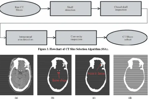
Figure 3. Flowchart of CT Slice Selection Algorithm (SSA).

(a) (b) (c) (d)

Figure 4. Skull detection process on CT slice No.19. (a) Raw CT slice, (b) the detected bones B by the threshold method, (c) he candidate skull bone Ca after removing small bone chips and (d) the detected skull.

(4)

After finding each of the components which does not- be



1, 2, ,



long to the skull, the area of these components is computed. Using the computed areas, only those connected regions with an area less than a set threshold S is considered as a hole within the bone structure of the original scan. For this study based on the relative sizes of the objects found in brain CT scans, S has been set to 200 pixels which is a fair estimate of possible hole size. Once these holes have been identified inside the candidate skull structure, they are filled with bone intensity (equal to 1 in binary the matrix). This helps unify the overall identified bone structure by covering all the holes. A subset of the inverted matrices which are identified as holes within the bone structure is given as Hk (k = 1, 2, ···,

q) to express the bone hole regions.

 

where M is the converted matrix defined

pection tected skull  by combining the candidate skull matrix (J

−M) with all whitened small holes matrices Lk as shown

−M) represents the candidate skull corresponding to the connected region Ca.

2.1.2. Closed Skull Ins

Followed by the skull detection

algorithm is the closed skull inspection. This process aims to remove the slices with either unclosed skull or with the skull containing too many separated regions. The non-integrated skull affects the following IML iden- tification since symmetry value calculation through the exhaustive symmetric position search process is sensitive to the skull contour.

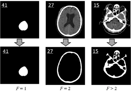
We define a new measure, called skull closing level F, using the number of zero matrices among all hole matrices Hk (k = 1, 2, ···, q).

candidate skull nor to the small bone hole. Therefore,

n generally has larger intracranial area, such as nce in this step, the

the detected skull. O

a binary state-variable used to express whether Hk is a

zero matrix. When Hk is a zero matrix, it means that the

kth connected-converted region D belongs neither to the

those zero matrices Hk should be the regions separated by

the detected skull  as the black regions either inside or outside the detected skull shown in the bottom three figures of Figure 5.

If the computed skull closing level F is equal to 2, it implies that the skull is integrated and ideal for the following steps of detection, such as slice No.27 shown in

Figure 5. However, if F is not equal to 2, it means that the image cannot be used in the detection of the ideal midline due to an inappropriate scan position, such as the slices No.41 and No.15 in Figure 5. The skull closing level measure can quantitatively evaluate the integrity of the skull in head CT images. After closed skull inspect- tion, all images with F  2 are removed from the slice subset.

2.1.3. Intracranial Area Detection

Based on clinical experience, the ideal CT slice for IML detectio

the slices No.22 - 30 in Figure 2. He

area of the inner region surrounded by the detected skull, namely the intracranial pixels, is calculated and sorted for all remaining slices in the subset.

In the subset of images acquired after the closed skull detection step, every CT image should contain only two black regions which are separated by

ne of them is the intracranial region which contains the mass center of the skull and the other is the region outside of the skull. In order to calculate the intracranial area, the intracranial region has to be distinguished from region outside of the skull. This can be achieved using the coordinate of the skull’s mass center.

Generally, the imagemoment mpq of the order p + q of

(5)

the digital image  can be defined as below, skull matrix . Then, the coordinate of the mas

(x, y) of the detected skull can be obtained by the coordinate of the skull mass

tracranial region. The intracranial area Sin of this image is

given by

The intracranial area of every slice in the subset is calculated and sorted in descending order. The first  slices with larger intracranial area a

following inspection. This number o de

re selected out for the f  is a variable that pends on the number of slices for one patient or physi-cian’s requirement. selected percentage of the whole num er of slices b . After experimenting with va

25% were finally chosen fo

e for IML detection is generally a good convexity for the intracranial cranial regions of the slices

extract the contour of the intracranial re

rious valu r this study.

es, γ = 10 and η =

2.1.4. Convexity Inspection

According to practical experience, another important characteristic of an ideal head CT imag

region. For instance, the intra

No.19 - 20 which are not ideal for IML detection both have integrated skull and larger intracranial area but show partially concavity. In contrast, intracranial regions of slices 26 through 28 have good convexity (see Figure 2). In addition, the concave shape of the intracranial region could affect the accuracy of the exhaustive symmetric position search, which is performed in the subsequent IML detection.

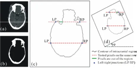
To qualitatively measure and evaluate the convexity of the intracranial region, we define a new measure Λ, called the intracranial convex measure. As shown in

Figure 6(c), we

gion. Then we can scan those pixels row by row. We define the far left and far right junctions (the blue points) of the ith row line (the upper red dash line) and the intracranial contour (the black curve) as points LPi and RPi

in Figure 6(c). We use the function ξ(i,j) to describe the

out-of-intracranial-region pixels between LPi and RPi on

the ith row as the green bold line shown in Figure 6(c).

where R represents the intracranial region. Then the number of the out-of-intracranial-region pixels on t row φ(i) is given as below

We define the intracranial convex measure Λ using the total number of the out-of-intracranial-region

all m rows of the image.

m

nial convex measure at angle φ can be calculated and noted as Λφ.

m

e rotated by angle φ. With the sum of the all Λφ at all rota

intracranial convex measure ΛTotal is

the in tracranial region in a CT image. Using the s

we can keep the better  CT slices in the slice-sub re

Figure 6(d). The intracra

 

1

i i

 _ _

 



 (20)

where Ψφ(i) the number of the out-of-intracranial-region pixels on the ith row in the imag

ting angles, the total given as below.

Larger values of the total intracranial convex measure ΛTotal represent increasingly worse convexity of

orted ΛTotal, set by moving the ones with worse convexity. Value of  can be decided by Equation (16). For the example under study, using γ = 6 and η = 15% around 6 slices were obtained for the slice subset after convexity inspection.

With the implementation of the SSA algorithm on the raw slices, the number of slices greatly decreases. For

(6)

nearly all the slices of the obtained SSA subset e ideal midline midline detection is a

0 0

ations (10) and (14), respectively. To find the ap- xhaustive symmet-

edge and the cur- re

instance, in the case of Figure 1, the slice number of this patient’s scans decreases from 42 to only 6. The reduc- tion in the number of slices effectively enhances the efficiency and saves computational time in the steps that follow.

2.2. Ideal Midline Detection

After the slice selection is performed using SSA algorithm,

are considered to be appropriate for th detection (IML detection). Ideal

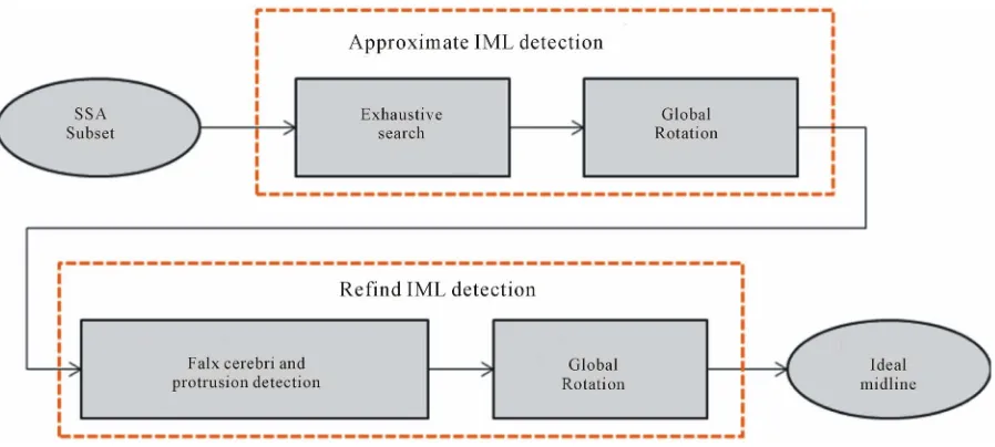
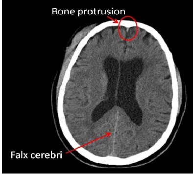
two- step procedure, which includes the detection of the approximate ideal midline and subsequently refining the detected ideal midline, as shown in Figure 7. In the first step, the ideal midline can be approximated based on the skull symmetry, however including other features of the skull and the brain can help improve the accuracy of the- approximation. Thus, in the refined IML detection step, the bone protrusion on the upper part of the skull and the falx cerebri in the lower part are used to accurately detect the position of the ideal midline. To fully consider the connection among the slices in the subset, we utilize a global rotation assumption in both steps to determine the rotation angle of the skull. This method can further reduce the detection error due to individual non-ideal image.

2.2.1. Approximate IML Detection

In the calculation of the SSA algorithm, the detected skull  and its mass center (x, y) have been determined

y Equ b

proximate ideal midline, we use the e

ric position search algorithm which was developed for a prior work by our research group [8].

The row symmetry is defined as the difference in di-

stance between each side of the skull

nt approximate midline. The CT image is rotated around the mass center of the skull. The symmetry cost Sθof the image at the rotation angle θis calculated as the sum of all row symmetry in the resulting image as shown in Equation (22).

1 i i i

 

m

S 



l r (22)

where m is the number of rows in th rotation angle θ (−45˚ < θ < +45˚ as u

e image with the sed in this study) and measure li and ri are the distance between the edge of

the skull on the left/right side and the current approxi-mate midline at the ith row. More details can be found in [8]. Finally, the rotation angle θ with the minimum sym-metry cost Sθ determines the rotation direction of the midline of the brain for each particular CT slice.

1 2

argmin , ,...,

p p pi

Rj

p S S S



 _  

  (23)

e on the pth where θp is the rotation angle of the midlin

slice and S

pi

 is the symmetry cost of the pth slice at

sl

e symmetric position search. How- ev

ngle of th

the rotation angle θpj.

All 6 CT ices in the SSA subset are processed one at a time using exhaustiv

er, due to the non-uniform-thickness of the skull to serious deformation of the skull on one side after injury, it is hard to get an accurate position of the midline by processing only one slice. In this work, a global rotation assumption is used to decide the approximate ideal midline of all the CT images from one patient with full con- sideration of the connection among all the slices.

In the global rotation assumption, we assume that all CT images of one patient have the same rotation a

e ideal midline due to the fixed posture of the patient during scanning. The rotation direction of the approxi-

(7)

mate ideal midline is determined by the median value of the rotation angles of all 6 slices in the SSA subset as shown below.

th termined by the exhaustive symmetric

pos  is the number of slices in the SSA

e approximate ideal midline of the lices. At the end of the approximate IML approximate ideal midline on each slice is ertical direction by rotating the skull by

2.2.2. Refined Ideal Midline Detection

Once the approximate midline is estimated and calibrated, brain anatomical features, such as the

The falx cerebri is a strong arched fold

that descends vertically in the longitudinal fissure be-

e, the derivative of the curve is calculated in been chosen to

position of the falx , are used to refine cerebri and protrusion of skull bone

the detection. In the detection of the falx cerebri and pro-trusion, we use the same algorithm from our previous work [8].

of dura mater

tween the left and right cerebral hemispheres (Figure 8). In this work, edge detection method and Hough trans- form are used to detect this anatomical feature quickly and accurately. On the other hand, a bone protrusion is located in the anterior section of the skull. As shown in

Figure 8, the bone protrusion curves down to a minimum

point which is considered to be the upper starting point of the falx cerebri. To locate the lowest point of the protrusion curv

a limited neighborhood area, which has

be 10 - 15 pixels in this work. The local minima point a is determined by the following equation.









 

argmax 2

a

x  _ x w   x w   x _ (25)

Figure 8. The falx cerebri and the bone protrusion.

where the function ( )x is the extracted curve of the interior bone edge and w is the neighborhood width. In fact, several small local minimal points may exist around the neighbor area of the protrusion due to the noise of the image or the irregularities of the skull. Using the maxi- mal second derivative of the curve as the point a, Equa- tion (25) is used to successfully extract the true protrusion minimal point by avoiding the influence of noise. More details of the detection of the falx cerebri and the bone protrusion can be found in [8].

Using the detected falx cerebri and the bone protrusion, we can obtain the refined rotation angle θq of the midline

on each slice. Again, the global rotation assumption is used to determine the refined ideal midline of the whole set of slices. Rather than using the median method in the approximate midline detection, the weighted aver ge method is used in this refine detection step. The rota on

ed ideal midline of all the slices is given by

where θq is the refined rotation angle of the midline on

the qth slice and μq is the weight of θq in the refined IML

detection calculation.

1

2

1 if the falx cerebri and protrusion are both detected

if only the falx cerebri is detected

0 if neither falx cerebri and protrusion is detected

q

At the end of the refined IML detection, the idea i-

dlin di-

re

aracteristics of the skull and closely simulates the process l m e on each slice is calibrated again to the vertical

e sk

c- tion by rotating th ull by −θf angle. Therefore, in

the two-step ideal midline detection, the ideal midline is centered by the mass center of the skull and rotated by an angle of −(θa + θf) from the original position in the slice.

3. Results and Discussion

3.1. Data

This database contains 3133 axial CT scan slices acquired across 70 patients with cases of both mild and severe Traumatic Brain Injuries (TBI). All the available CT scans have been utilized in testing the system’s proc- esses and in the estimation of ideal midline.

3.2. Experimental Results and Discussion

(8)

m

ur method is only 2.1 pixels, which is much less than the ones reported in [1,8,10]. The above experimental results demonstrate the high reliability of the proposed system.

4. Summary

In this paper, we proposed a system to identify the ideal midline (IML) using CT scans of patients with head injuries. The proposed SSA algorithm is used to closely si- mulate the process of manual selection of CT slice by

ing

th to

ro mption fully considers the connection am-

ong CT slices and thereb mpens s the erro ner-

ated by slice. The obtained results

u syste be impl ted

in clin

CE

[ Ruppert, L. Teverovskiyz, C. Yu, A. X. Falcao,

L N mmetr Based Method for

l Plane Extraction in Neuroimages,” IEEE In-ona sium edical Imaging, Chicago,

2011, pp. 285-288.

[2] roder ad Computed To aphy Inte tation

of manual CT slice selection and decision making in IML by physicians.

In our dataset, all CT slices selected out by the SSA algorithm have been found to be acceptable for use in IML detection with the physician’s

stance, the patient in Figure 1 has 42

CT scan. With the implementation of the SSA algorithm,

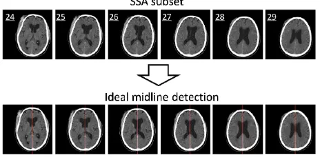
the IML detection step due to the features such as integrated skull, large intracranial area, and good convexity of the skull. The result of the IML detection is displayed in the lower images of Figure 9. We can see that the detected ideal midline is accurately located in the middle of the skull and that the skulls in each scan are calibrated correctly.

m

confirming. For in- raw CT slices after

only 6 slices were selected to be in the SSA subset as shown in the upper figures in Figure 9. All 6 slices are found to be ideal for

In order to quantitatively easure the performance of the proposed system, the collaborating physician manually estimated IML is used as the ground truth. With a strict definition of accuracy, which is an allowed error of three pixels in horizontal distance δ between the estimated IML and the ground truth, the accuracy of IML estimation in this system is 96.9%

, which is h

igher than 95% reported in [8]. In order to evaluate the result of the

per fig-Figure 9. The results of the SSA algorithm (the up ures) and the ideal midline detection (the lower figures).

Table 1. Comparison on the accuracy of IML estimation.

Method Our method Chen, [8] Ruppert, [1] Teverovskiy, [10] Number of

id-sagittal plane estimation, Ruppert et al. used an average z-distance measure to indicate the displacement between the resulting plane and the ground truth plane inside one image [1]. Therefore, the average z-distance measure has the similar physical meaning as the error δin our method. The lesser the mean value of error δ, the closer the estimated IML is to the ground truth. As the comparison in Table 1, the mean value of the error δin o

physicians. With the implementation of SSA, a vast re- duction can be achieved of the number of slices that is

sed for the computation of IML detection steps. Hav u

fewer and more appropriate slices effectively increases e efficiency of the algorithm and also has the potential save the cost and time required in practice. The global tation assu

ternati l Sympo on Biom

30 March

J. S. B , “He mogr rpre

in Trauma: A Primer,” The Psychiatric Clinics of North America, Vol. 33, No. 4, 2010, pp. 821-854.

doi:10.1016/j.psc.2010.08.006

[3] Q. Hu and W. L. Nowinski, “A Rapid Algorithm for Ro-bust and Automatic Extraction of the Midsagittal Plane of the Human Cerebrum from Neuroimages Based on Local Symmetry and Outlier Removal,” NeuroImage, Vol. 20, No.4, 2003, pp. 2153-2165.

doi:10.1016/j.neuroimage.2003.08.009

[4] C. C. Liao, F. Xiao, J. Wong, and I. Chiang, “A Simple Genetic Algorithm for Tracing the Deformed Midline on a Single Slice of Brain CT Using Quadratic Bezier Cur- ves,” Sixth IEEE International Conference on Data Min-ing Workshops, Hong Kong, 18-22 December 2006, pp. 463-467. doi:10.1109/ICDMW.2006.22

o, G. C. S. Ruppert and A. X. Falcao, “Fast [5] F. P. G. Berg

(9)

Bioin-spired Systems and Signal Processing, 2008, pp. 92-99. [6] R. Guillemaud, P. Marais, A. Zisserman, B. McDonald, T.

J. Crow and M. Brady, “A Three Dimensional Mid-Sagit-tal Plane for Brain Asymmetry Measurement,” Schizo-phrenia Research, Vol. 18, No. 2, 1996, pp. 183-184. doi:10.1016/0920-9964(96)85575-7

[7] W. Chen, R. Smith, S. Y. Ji and K. Najarian, “Automated Segmentation of Lateral Ventricales in Brain CT Images,”

IEEE International Conference on Bioinformatics and Biomeidcine Workshops, Philadelphia, 3-5 November 2008, pp. 48-55.

[8] W. Chen, R. Smith, S. Y. Ji, K. Ward and K. Najarian, “Automated Ventricular Systems Segmentation in Brain CT Images by Combining Low-Level Segmentation and

High-Level Template Matching,” BMC Medical Infor-matics and Decision Making, Vol. 9, No. 1, 2009, p. S4. doi:10.1186/1472-6947-9-S1-S4

[9] R. M. Haralick and L. G. Shapiro, “Computer and Robot Vision,”1992.