Chapter 2
2
Introduction
• Many management decisions involve trying to make the most effective use of an organization’s resources.
• Resources typically include machinery, labor, money, time, warehouse space, or raw materials.
• Resources may be used to produce products (such as
machinery, furniture, food, or clothing) or services (such as schedules for shipping and production, advertising policies, or investment decisions).
• Linear programming (LP) is a widely used mathematical technique designed to help managers in planning and
decision making relative to resource allocation.
• Despite the name, linear programming, and the more general category of techniques called “mathematical programming”, have very little to do with computer programming.
• In the world of Operations Research, programming refers to
modeling and solving a problem mathematically.
Most of the deterministic OR models can be formulated as mathematical programs.
"Program," in this context, has to do with a “plan,” not a computer program.
General form of Linear programming model
Maximize / Minimize z = f(x1, x2 ,…, xn)
Subject to
{
}
b i i =1,…,m
xj ≥ 0, j = 1,…,n
Linear Programming Model
4
• xj are called decision variables. These are
things that you control and you want to determine its values
{
}
biare called structural
(or functional or technological) constraints
• xj ≥ 0 are nonnegativity constraints
Model Components
• f(x1, x2 ,…, xn) is the objective function
Example: Giapetto woodcarving Inc.,
• Giapetto Woodcarving, Inc., manufactures two types of wooden toys: soldiers and trains. A soldier sells for $27 and uses $10 worth of raw materials. Each soldier that is manufactured increases Giapetto’s variable
labor and overhead cost by $14. A train sells for $21 and uses $9 worth of raw materials. Each train built increases Giapetto’s variable labor and overhead cost by $10. The manufacture of wooden soldiers and
trains requires two types of skilled labor: carpentry and finishing. A soldier requires 2 hours of finishing labor and 1 hour of carpentry labor. A train requires 1 hour of finishing and 1 hour of carpentry labor. Each week, Giapetto can obtain all the needed raw material but only 100 finishing hours and 80 carpentry hours. Demand for trains is unlimited, but at most 40
soldiers are bought each week. Giapetto wants to maximize weekly profit. Formulate a linear
6
Solution: Giapetto woodcarving Inc.,
• Step 1: Model formulation
1. Decision variables: we begin by finding the
decision variables. In any LP, the decision variables should completely describe the decisions to be made. Clearly, Giapetto
must decide how many soldiers and trains should be manufactured each week. With this in mind, we define:
X1 = number of soldiers produced each
week
X2 = number of trains produced each
7
Solution: Giapetto woodcarving Inc.,
2. Objective function: in any LP, the decision
maker wants to maximize (usually revenue or profit) or minimize (usually costs) some function of the decision variables. The
function to be maximized or minimized is called the objective function. For the
Giapetto problem, we will maximize the net profit (weekly revenues – raw materials cost – labor and overhead costs).
Weekly revenues and costs can be expressed in terms of the decision variables, X1 and X2
8
Solution: Giapetto woodcarving Inc.,
• Weekly revenues = weekly revenues from soldiers + weekly revenues from trains
= 27 X1 + 21 X2
Also,
Weekly raw materials costs = 10 X1 + 9 X2
Other weekly variable costs = 14 X1 + 10 X2
Therefore, the Giapetto wants to maximize:
(27 X1 + 21 X2) – (10 X1 + 9 X2) – (14 X1 + 10 X2)
= 3 X1 + 2 X2
Hence, the objective function is:
Solution: Giapetto woodcarving Inc.,
3. Constraints: as X1 and X2 increase,Giapetto’s objective function grows larger. This means that if Giapetto were free to
choose any values of X1 and X2, the
company could make an arbitrarily large profit by choosing X1 and X2 to be very
large. Unfortunately, the values of X1 and X2
are limited by the following three
restrictions (often called constraints):
Constraint 1: each week, no more than 100
hours of finishing time may be used.
Constraint 2: each week, no more than 80
hours of carpentry time may be used.
Constraint 3: because of limited demand, at
10
Solution: Giapetto woodcarving
Inc.,
• The three constraints can be expressed in terms of the decision variables X1 and X2 as
follows:
Constraint 1: 2 X1 + X2 100
Constraint 2: X1 + X2 80
Constraint 3: X1 40
Note:
The coefficients of the decision variables in the constraints are called technological
coefficients. This is because its often reflect
the technology used to produce different
products. The number on the right-hand side of each constraint is called Right-Hand Side
(RHS). The RHS often represents the quantity
11
Solution: Giapetto woodcarving Inc.,
• Sign restrictions: to complete the formulation
of the LP problem, the following question
must be answered for each decision variable: can the decision variable only assume
nonnegative values, or it is allowed to
assume both negative and positive values?
If a decision variable Xi can only assume a
nonnegative values, we add the sign
restriction (called nonnegativity constraints) Xi 0.
If a variable Xi can assume both positive and negative values (or zero), we say that Xi is
unrestricted in sign (urs).
12
Solution: Giapetto woodcarving Inc.,
• Combining the nonnegativity
constraints with the objective function
and the structural constraints yield the
following optimization model (usually
called LP model):
Max Z = 3 X1 + 2 X2 (objective function)
subject to (st)
2 X1 + X2 100 (finishing constraint)
X1 + X2 80 (carpentry constraint)
X1 40 (soldier demand constraint)
X1 0 and X2 0 (nonnegativity constraint)
The optimal solution to this problem is :
13
What is Linear programming
problem (LP)?
• LP is an optimization problem for which we do the
following:
1. We attempt to maximize (or minimize) a linear
function of the decision variables. The function that is to be maximized or minimized is called objective function.
2. The values of decision variables must satisfy a set of constraints. Each constraint must be a linear
equation or linear inequality.
3. A sign restriction is associated with each variable. for any variable Xi, the sign restriction specifies
either that Xi must be nonnegative (Xi > 0) or that Xi
14
Linear Programming Assumptions
(i) proportionality
(ii) additivity linearity
(iii) divisibility
(i) activity j’s contribution to objective function is
cjxj
and usage in constraint i is aijxj
both are proportional to the level of activity j
(volume discounts, set-up charges, and nonlinear efficiencies are potential sources of violation)
(ii) “cross terms” such as x1x5 may not appear in the objective or constraints.
16
(iii) Fractional values for decision variables are permitted
(iv) Data elements aij , cj , bi , uj are known with certainty
• Nonlinear or integer programming models should be used when some subset of assumptions (i), (ii) and (iii) are not satisfied.
• Stochastic models should be used when a problem has significant uncertainties in the data that must be explicitly taken into account [a relaxation of assumption (iv)].
Applications Of LP
1. Product mix problem 2. Diet problem
3. Blending problem
4. Media selection problem 5. Assignment problem
6. Transportation problem
7. Portfolio selection problem 8. Work-scheduling problem
9. Production scheduling problem 10. Inventory Problem
18
1. Product Mix Problem
Example
Formulate a linear programming model for this problem, to determine how many containers of each product to produce tomorrow in order to maximize the profits. The company makes four types of juice using orange, grapefruit, and
pineapple. The following table shows the price and cost per quart of juice (one container of
juice) as well as the number of kilograms of fruits required to produce one quart of juice.
Product Price/quart Cost/quart Fruit needed
Orange juice 3 1 1 Kg.
Grapefruit juice 2 0.5 2 Kg.
Pineapple juice 2.5 1.5 1.25 Kg.
Example (cont.)
On hand there are 400 Kg of orange, 300 Kg. of grapefruit, and 200 Kg. of pineapples.
The manager wants grapefruit juice to be used for no more than 30 percent of the
number of containers produced. He wants the ratio of the number of containers of orange
juice to the number of containers of pineapples juice to be at least 7 to 5.
pineapples juice should not exceed one-third of the total product.
20
Product Mix Problem
Solution
Decision variables
X1 = # of containers of orange juice X2 = # of containers of grapefruit juice X3 = # of containers of pineapple juice X4 = # of containers of All-in-one juice Objective function
Ratio of orange to pineapple Max. of pineapple
21
2. Diet problem
Example
My diet requires that all the food I eat come from one of the four “basic food groups” (chocolate cake, ice cream, soda, and cheesecake). At present, the
following four foods are available for consumption: brownies, chocolate ice cream, cola, and pineapple cheesecake. Each brownie costs 50 cents, each
scoop of chocolate ice cream costs 20 cents, each bottle of cola costs 30 cents, and each piece of
pineapple cheesecake costs 80 cents. Each day, I must ingest at least 500 calories, 6 oz of chocolate, 10 oz of sugar, and 8 oz of fat. The nutritional
content per unit of each food is shown in the
following table. Formulate a linear programming model that can be used to satisfy my daily
22
Diet problem
Calories Chocolat
e Sugar Fat
Brownie 400 3 ounce 2 ounce 2 ounce
Chocolate ice cream (1 scoop)
200 2 2 4
Cola (1 bottle) 150 0 4 1
Pineapple cheesecake
23
Diet
problem
Solution
• Decision variables: as always, we begin by
determining the decisions that must be made by the decision maker: how much of each
food type should be eaten daily. Thus, we define the decision variables:
X1 = number of brownies eaten daily
X2 = number of scoops of chocolate ice cream
eaten daily
X3 = number of bottles of cola drunk daily
X4 = number of pieces of pineapple cheesecake
24
Diet problem
• Objective function:
my objective
function is to minimize the cost of my
diet. The total cost of my diet may be
determined from the following relation:
Total cost of diet = (cost of brownies) +
(cost of ice cream) + (cost of cola) +
(cost of cheesecake)
Thus, the objective function is:
25
Diet problem
• Constraints: the decision variables must satisfy the following four constraints:
Constraint 1: daily calorie intake must be at least 500 calories.
Constraint 2: daily chocolate intake must be at least 6 oz.
Constraint 3: daily sugar intake must be at least 10 oz.
Constraint 4: daily fat intake must be at least 8 oz. To express constraint 1 in terms of the decision
variables, note that (daily calorie intake) = (calorie in brownies) + (calories in chocolate ice cream) +
(calories in cola) + (calories in pineapple cheesecake) Therefore,
the daily calorie intake = 400 X1 + 200 X2 + 150 X3 +
500 X4 must be greater than 500 ounces
26
Diet problem
The four constraints are:
400 X
1+ 200 X
2+ 150 X
3+ 500 X
4
500
3 X
1+ 2 X
2
6
2 X
1+ 2 X
2+ 4 X
3+ 4 X
4
10
2 X
1+ 4 X
2+ X
3+ 5 X
4
8
Nonnegativity constraints:
it is clear that
all decision variables are restricted in
sign, i.e., X
i
0, for all i = 1, 2, 3, and
Diet problem
• Combining the objective function,
constraints, and nonnegativity constraints, the LP model is as follows:
Min Z = 50 X1 + 20 X2 + 30 X3 + 80 X4
st.
400 X1 + 200 X2 + 150 X3 + 500 X4 500
3 X1 + 2 X2 6
2 X1 + 2 X2 + 4 X3 + 4 X4 10
2 X1 + 4 X2 + X3 + 5 X4 8
Xi 0, for all i = 1, 2, 3, and 4
The optimal solution to this LP is X1 = X4 = 0,
28
3. Blending problem
Example
The Low Knock Oil company produces two grades of cut rate gasoline for industrial distribution. The grades, regular and economy, are
produced by refining a blend of two types of crude oil, type X100 and type X220. each crude oil differs not only in cost per barrel, but in composition as well. The accompanying table indicates the
percentage of crucial ingredients found in each of the crude oils and the cost per barrel for each. Weekly demand for regular grade of Low Knock gasoline is at least 25000 barrels, while demand for the
economy is at least 32000 barrels per week. At least 45% of each barrel of regular must be ingredient A. At most 50% of each barrel of economy should contain ingredient B. the Low Knock management must decide how many barrels of each type of crude oil to buy each week for blending to satisfy demand at minimum cost .
Crude oil
type Ingredient A % Ingredient B % Cost/barrel ($)
X100 35 55 30
Blending problem
Solution
Let
X1 = # of barrels of crude X100 blended to produce the refined regular
X2 = # of barrels of crude X100 blended to produce the refined economy
X3 = # of barrels of crude X220 blended to produce the refined regular
X4 = # of barrels of crude X220 blended to produce the refined economy
Min Z = 30 X1 + 30 X2 + 34.8 X3 + 34.8 X4
St.
X1 + X3 25000
X2 + X4 32000
-0.10 X1 + 0.15 X3 0
0.05 X2 – 0.25 X4 0
Xi 0, i = 1, 2, 3, 4
The optimal solution is: X1 = 15000, X2 = 26666.6, X3 = 10000,
30
4. Media selection problem
Example
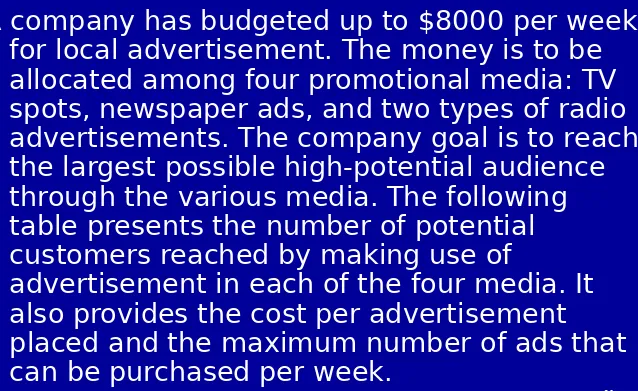
A company has budgeted up to $8000 per week for local advertisement. The money is to be
allocated among four promotional media: TV spots, newspaper ads, and two types of radio advertisements. The company goal is to reach the largest possible high-potential audience through the various media. The following
table presents the number of potential customers reached by making use of
advertisement in each of the four media. It also provides the cost per advertisement
31
TV spot (1 minute) 5000 800 12
Daily newspaper
The company arrangements require that at least five radio spots be placed each week. To ensure a board-scoped promotional
32
Media selection
Solution
Let
X1 = number of 1-miute TV spots taken Each week
X2 = number of full-page daily newspaper ads taken each week.
X3 = number of 30-second prime-time radio spots taken each week.
X4 = number of 1-minute afternoon radio spots taken each week.
Max Z = 5000 X1 + 8500 X2 + 2400 X3 + 2800 X4
st
X1 12 (maximum TV spots/week)
X2 5 (maximum newspaper ads/week)
X3 25 (maximum 30-second radio spots/week)
X4 20 (maximum 1-minute radio spots/week)
800 X1 + 925 X2 + 290 X3 + 380 X4 8000 (weekly budget)
X3 + X4 5 (minimum radio spots contracted)
290 X3 + 380 X4 1800 (maximum dollars spent on radio)
X1, X2, X3, X4 0
33
5. Assignment problem
Example
A law firm maintains a large staff of young attorneys who hold the title of junior partner. The firm
concerned with the effective utilization of this
personnel resources, seeks some objective means of making lawyer-to-client assignments. On march 1, four new clients seeking legal assistance came to the firm. While the current staff is overloads and identifies four junior partners who, although busy, could possibly be assigned to the cases. Each young lawyer can handle at most one new client.
Furthermore each lawyer differs in skills and specialty interests.
Seeking to maximize the overall effectiveness of the new client assignment, the firm draws up the
following table, in which he rates the estimated
34
Assignment problem
Client case
Lawyer Divorce Corporate
merger embezzlement exhibitionism
Adam 6 2 8 5
Brook 9 3 5 8
Carter 4 8 3 4
Assignment problem
Solution
Decision variables:
1 if attorney i is assigned to case j Let Xij =
0 otherwise
Where : i = 1, 2, 3, 4 stands for Adam, Brook, Carter, and Darwin respectively
j = 1, 2, 3, 4 stands for divorce,
merger, embezzlement, and exhibitionism respectively.
36
Assignment problem
Max Z = 6 X11 + 2 X12 + 8 X13 + 5 X14 + 9 X21 + 3 X22 +
5 X23 + 8 X24 + 4 X31 + 8 X32 + 3 X33 + 4 X34 +
6 X41 +7 X42 + 6 X43 + 4 X44
St.
X11 + X21 + X31 + X41 = 1 (divorce case)
X12 + X22 + X32 + X42 = 1 (merger)
X13 + X23 + X33 + X43 = 1 (embezzlement)
X14 + X24 + X34 + X44 = 1 (exhibitionism)
X11 + X12 + X13 + X14 = 1 (Adam)
X21 + X22 + X23 + X24 = 1 (Brook)
X31 + X32 + X33 + X34 = 1 (Carter)
X41+ X42 + X43 + X44 = 1 (Darwin)
The optimal solution is: X13 = X24 = X32 = X41 = 1. All other variables are equal to zero.
6. Transportation problem
Example
The Top Speed Bicycle Co. manufactures and markets a line of 10-speed bicycles nationwide. The firm has
final assembly plants in two cities in which labor costs are low, New Orleans and Omaha. Its three major
warehouses are located near the larger market areas of New York, Chicago, and Los Angeles.
The sales requirements for next year at the New York warehouse are 10000 bicycles, at the Chicago
warehouse 8000 bicycles, and at the Los Angeles warehouse 15000 bicycles. The factory capacity at each location is limited. New Orleans can assemble and ship 20000 bicycles; the Omaha plant can
produce 15000 bicycles per year. The cost of shipping one bicycle from each factory to each warehouse
38
Transportation problem
New
York Chicago AngeleLos
s
New Orleans $2 3 5
Omaha 3 1 4
39
Transportation problem
Solution
To formulate this problem using LP, we again employ the concept of double subscribed variables. We let the
first subscript represent the origin (factory) and the second subscript the destination (warehouse). Thus, in general, Xij refers to the number of bicycles shipped
from origin i to destination j. Therefore, we have six
decision variables as follows:
X11 = # of bicycles shipped from New Orleans to New York
X12 = # of bicycles shipped from New Orleans to Chicago
X13 = # of bicycles shipped from New Orleans to Los Angeles
X21 = # of bicycles shipped from Omaha to New York X22 = # of bicycles shipped from Omaha to Chicago
40
Transportation problem
Min Z = 2 X11 + 3 X12 + 5 X13 + 3 X21 + X22 + 4
X23
St
X11 + X21 = 10000 (New York demand)
X12 + X22 = 8000 (Chicago demand)
X13 + X23 = 15000 (Los Angeles demand)
X11 + X12 + X13 20000 (New Orleans Supply
X21 + X22 + X23 15000 (Omaha Supply)
Xij 0 for i = 1, 2 and j = 1, 2, 3
The optimal solution is: X11 = 10000, X12 = 0, X13 = 8000, X21 =
7. Portfolio selection
Example
The International City Trust (ICT) invests in short-term trade credits, corporate bonds, gold
stocks, and construction loans. To encourage a diversified portfolio, the board of directors has placed limits on the amount that can be
committed to any one type of investment. The ICT has $5 million available for immediate
investment and wishes to do two things: (1) maximize the interest earned on the
42
Portfolio selection
Investment Interest
earned %
Maximum investment
($ Million)
Trade credit 7 1
Corporate bonds 11 2.5
Gold stocks 19 1.5
Construction loans 15 1.8
In addition, the board specifies that at least 55% of the funds invested must be in gold
Portfolio selection
Solution
To formulate ICT’s investment problem
as a linear programming model, we
assume the following decision
variables:
X
1= dollars invested in trade credit
X
2= dollars invested in corporate bonds
X
3= dollars invested in gold stocks
X
4= dollars invested in construction
44
Portfolio selection
Max Z = 0.07 X1 + 0.11 X2 + 0.19 X3 + 0.15 X4
St.
X1 1
X2 2.5
X3 1.5
X4 1.8
X3 + X4 0.55(X1 + X2 + X3 + X4)
X1 0.15(X1 + X2 + X3 + X4)
X1 + X2 + X3 + X4 5
Xi 0 , i = 1, 2, 3, 4
The optimal is: X1 = 75,000, X2 = 950,000, X3 =
1,500,000, and X4 = 1,800,000, and total interest
45
8. Work Scheduling Problem
Example
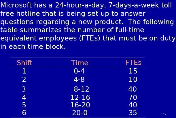
Microsoft has a 24-hour-a-day, 7-days-a-week toll free hotline that is being set up to answer
questions regarding a new product. The following table summarizes the number of full-time
equivalent employees (FTEs) that must be on duty in each time block.
Shift Time FTEs
1 0-4 15
2 4-8 10
3 8-12 40
4 12-16 70
5 16-20 40
46
• Microsoft may hire both full-time and part-time
employees. The former work 8-hour shifts and the latter work 4-hour shifts; their respective hourly
wages are $15.20 and $12.95. Employees may start work only at the beginning of one of 6 shifts.
Part-time employees can only answer 5 calls in the time a full-time employee can answer 6 calls. (i.e., a part-time employee is only 5/6 of a full-time
employee.)
Formulate an LP to determine how to staff the hotline at minimum cost.
Decision Variables
PT employee is 5/6 FT employee
48
Terminology for solution of LP
• A feasible solution is a solution for which all the constraints are satisfied.
• A corner point feasible solution (CPF) is a feasible solution that lies at a corner point. • An infeasible solution is a solution for which
at least one constraint is violated.
• The feasible region is the collection of all feasible solution.
• An Optimal solution is a feasible solution that has the most favorable value of the objective function. (it is always one of the CPF solution • The most favorable value is the largest
Graphical solution
A Graphical Solution Procedure (LPs with 2 decision variables can be solved/viewed this way.)
1. Plot each constraint as an equation and then decide which
side of the line is feasible (if it’s an inequality).
2. Find the feasible region.
3. find the coordinates of the corner (extreme) points of the feasible
region.
4. Substitute the corner point coordinates in the objective
function
50
Example 1: A Minimization Problem
• LP Formulation
Min
z
= 5
x
1+ 2
x
2s.t. 2
x
1+ 5
x
2> 1
4
x
1-
x
2> 12
x
1+
x
2> 4
Example 1: Graphical Solution
• Graph the Constraints
• Constraint 1: When x1 = 0, then x2 = 2; when x2
= 0, then x1 = 5. Connect (5,0) and (0,2). The
">" side is above this line.
• Constraint 2: When x2 = 0, then x1 = 3. But
setting x1 to 0 will yield x2 = -12, which is not on
the graph. Thus, to get a second point on this
line, set x1 to any number larger than 3 and
solve for x2: when x1 = 5, then x2 = 8. Connect
(3,0) and (5,8). The ">" side is to the right.
• Constraint 3: When x1 = 0, then x2 = 4; when x2
= 0, then x1 = 4. Connect (4,0) and (0,4). The
52
Example 1: Graphical Solution
53
Example 1: Graphical Solution
• Solve for the Extreme Point at the Intersection of the second and third Constraints
4x1 - x2 = 12
x1+ x2 = 4
Adding these two equations gives:
5x1 = 16 or x1 = 16/5.
Substituting this into x1 + x2 = 4 gives: x2 = 4/5
• Solve for the extreme point at the intersection of the first and third constraints 2x1 + 5x2 =10
x1 + x2= 4
Multiply the second equation by -2 and add to the first equation, gives 3x2 = 2 or x2 = 2/3
Substituting this in the second equation gives x1 = 10/3
Point Z
(16/5, 4/5) 88/5
(10/3, 2/3) 18
54
Example 2: A Maximization Problem
Max
z
= 5
x
1+ 7
x
2s.t.
x
1< 6
2
x
1+ 3
x
2< 19
x
1+
x
2< 8
56
58
Example 2: A Maximization Problem
60
Example 2: A Maximization Problem
• The Five Extreme Points
Example 2: A Maximization Problem
• Having identified the feasible region for the problem, we now search for the optimal
solution, which will be the point in the
feasible region with the largest (in case of maximization or the smallest (in case of
minimization) of the objective function. • To find this optimal solution, we need to
62
Example 2: A Maximization Problem
Extreme Points and the Optimal Solution
• The corners or vertices of the feasible region are referred to as the extreme points.
• An optimal solution to an LP problem can be found at an extreme point of the feasible
region.
• When looking for the optimal solution, you do not have to evaluate all feasible solution
points.
64
Feasible Region
• The feasible region for a two-variable linearprogramming problem can be nonexistent, a single point, a line, a polygon, or an unbounded area.
• Any linear program falls in one of three categories: – is infeasible
– has a unique optimal solution or alternate optimal solutions
– has an objective function that can be increased without bound
Special Cases
• Alternative Optimal SolutionsIn the graphical method, if the objective function line is parallel to a boundary constraint in the
direction of optimization, there are alternate optimal solutions, with all points on this line segment being optimal.
• Infeasibility
A linear program which is overconstrained so that no point satisfies all the constraints is said to be infeasible.
• Unbounded
For a max (min) problem, an unbounded LP occurs in it is possible to find points in the feasible
66
Example with Multiple Optimal
Solutions
1 0
0 1
x
1
x
2
2 3 4 2
3 4
z
1 z2 z3
Maximize z = 3x1 – x2
subject to 15x1 – 5x2 30 10x1 + 30x2 120
Example: Infeasible Problem
• Solve graphically for the optimal solution:
Max z = 2x1 + 6x2
s.t. 4x1 + 3x2 < 12
2x1 + x2 > 8
68
Example: Infeasible Problem
• There are no points that satisfy both
constraints, hence this problem has no feasible region, and no optimal solution.
x
x22
x
x11
4
4xx11 + 3 + 3xx22 << 12 12 2
2xx11 + + xx22 >> 8 8
3
3 44 4
4
8
Example: Unbounded Problem
• Solve graphically for the optimal solution:
Max z = 3x1 + 4x2
s.t. x1 + x2 > 5
3x1 + x2 > 8
70
Example: Unbounded
Problem
• The feasible region is unbounded and the objective function line can be moved parallel to itself without bound so that z can be increased infinitely.
Solve the following LP graphically
Where x1 is the quantity produced
72
The graphical solution
( 1 )
Assignment: Complete the
problem to find the optimal solution E
Possible Outcomes of an LP
1. Infeasible – feasible region is empty; e.g., if the constraints include
x1+ x2 6 and x1+ x2
7
2. Unbounded - Max 15x1+ 7x2 (no finite optimal solution)
s.t.
3. Multiple optimal solutions - max 3x1 + 3x2
s.t. x1+ x2 1
x1, x2 0
4. Unique Optimal Solution
Note: multiple optimal solutions occur in many practical (real-world) LPs.
x1 + x2 1