Deep Belief
Nets in C++
and CUDA C:
Volume 3
Convolutional Nets
—
Deep Belief Nets in C++
and CUDA C: Volume 3
Convolutional Nets
ISBN-13 (pbk): 978-1-4842-3720-5 ISBN-13 (electronic): 978-1-4842-3721-2 https://doi.org/10.1007/978-1-4842-3721-2
Library of Congress Control Number: 2018940161
Copyright © 2018 by Timothy Masters
This work is subject to copyright. All rights are reserved by the Publisher, whether the whole or part of the material is concerned, specifically the rights of translation, reprinting, reuse of illustrations, recitation, broadcasting, reproduction on microfilms or in any other physical way, and transmission or information storage and retrieval, electronic adaptation, computer software, or by similar or dissimilar methodology now known or hereafter developed.
Trademarked names, logos, and images may appear in this book. Rather than use a trademark symbol with every occurrence of a trademarked name, logo, or image we use the names, logos, and images only in an editorial fashion and to the benefit of the trademark owner, with no intention of infringement of the trademark.
The use in this publication of trade names, trademarks, service marks, and similar terms, even if they are not identified as such, is not to be taken as an expression of opinion as to whether or not they are subject to proprietary rights.
While the advice and information in this book are believed to be true and accurate at the date of publication, neither the authors nor the editors nor the publisher can accept any legal responsibility for any errors or omissions that may be made. The publisher makes no warranty, express or implied, with respect to the material contained herein.
Distributed to the book trade worldwide by Springer Science+Business Media New York, 233 Spring Street, 6th Floor, New York, NY 10013. Phone 1-800-SPRINGER, fax (201) 348-4505, e-mail [email protected], or visit www.springeronline.com. Apress Media, LLC is a California LLC and the sole member (owner) is Springer Science + Business Media Finance Inc (SSBM Finance Inc). SSBM Finance Inc is a Delaware corporation.
For information on translations, please e-mail [email protected]; for reprint, paperback, or audio rights, please email [email protected].
Apress titles may be purchased in bulk for academic, corporate, or promotional use. eBook versions and licenses are also available for most titles. For more information, reference our Print and eBook Bulk Sales web page at www.apress.com/bulk-sales.
Any source code or other supplementary material referenced by the author in this book is available to readers on GitHub via the book’s product page, located at www.apress.com/9781484237205. For more detailed information, please visit www.apress.com/source-code.
Printed on acid-free paper Timothy Masters
Chapter 1: Feedforward Networks ... 1
Review of Multiple-Layer Feedforward Networks ... 1
Wide vs. Deep Nets ... 4
Locally Connected Layers ... 6
Rows, Columns, and Slices ... 7
Convolutional Layers ... 8
Half-Width and Padding ... 9
Striding and a Useful Formula ... 12
Pooling Layers ... 14
Pooling Types ... 14
The Output Layer ... 15
SoftMax Outputs ... 15
Back Propagation of Errors for the Gradient ... 18
Chapter 2: Programming Algorithms ... 23
Model Declarations ... 24
Order of Weights and Gradient ... 25
Initializations in the Model Constructor ... 26
Finding All Activations ... 29
Activating a Fully Connected Layer ... 30
Activating a Locally Connected Layer ... 31
Table of Contents
About the Author ... vii
About the Technical Reviewer ... ix
Activating a Convolutional Layer ... 34
Activating a Pooling Layer ... 36
Evaluating the Criterion ... 39
Evaluating the Gradient ... 42
Gradient for a Fully Connected Layer ... 46
Gradient for a Locally Connected Layer ... 48
Gradient for a Convolutional Layer ... 51
Gradient for a Pooled Layer (Not!) ... 52
Backpropagating Delta from a Nonpooled Layer ... 53
Backpropagating Delta from a Pooled Layer ... 56
Multithreading Gradient Computation ... 58
Memory Allocation for Threading ������������������������������������������������������������������������������������������ 63
Chapter 3: CUDA Code ... 67
Weight Layout in the CUDA Implementation ... 68
Global Variables on the Device ... 69
Initialization ... 71
Copying Weights to the Device ... 72
Activating the Output Layer ... 79
Activating Locally Connected and Convolutional Layers ... 81
Using Shared Memory to Speed Computation ����������������������������������������������������������������������� 88 Device Code ��������������������������������������������������������������������������������������������������������������������������� 93 Launch Code ... 99
Activating a Pooled Layer ... 101
SoftMax and Log Likelihood by Reduction ... 105
Computing Delta for the Output Layer ... 109
Backpropagating from a Fully Connected Layer ... 111
Backpropagating from Convolutional and Local Layers ... 113
Backpropagating from a Pooling Layer ... 119
Flattening the Convolutional Gradient ��������������������������������������������������������������������������������� 129
Launch Code for the Gradient ... 131
Fetching the Gradient ... 135
Putting It All Together ... 141
Chapter 4: CONVNET Manual ... 147
Menu Options ... 147
File Menu ����������������������������������������������������������������������������������������������������������������������������� 147 Test Menu ���������������������������������������������������������������������������������������������������������������������������� 149 Display Menu ... 150
Read Control File ... 150
Making and Reading Image Data ���������������������������������������������������������������������������������������� 151 Reading a Time Series as Images ��������������������������������������������������������������������������������������� 151 Model Architecture �������������������������������������������������������������������������������������������������������������� 155 Training Parameters ������������������������������������������������������������������������������������������������������������ 156 Operations ... 159
Display Options ... 160
Display Training Images ������������������������������������������������������������������������������������������������������ 160 Display Filter Images ����������������������������������������������������������������������������������������������������������� 160 Display Activation Images���������������������������������������������������������������������������������������������������� 161 Example of Displays ... 162
The CONVNET.LOG file ... 166
Printed Weights ... 169
The CUDA.LOG File ... 172
About the Author
Timothy Masters earned a PhD in mathematical statistics with a specialization in numerical computing in 1981. Since then he has continuously worked as an independent consultant for government and industry. His early research involved automated feature detection in high-altitude photographs while he developed applications for flood and drought prediction, detection of hidden missile silos, and identification of threatening military vehicles. Later he worked with medical researchers in the development of computer algorithms for distinguishing between benign and malignant cells in needle biopsies. For the past 20 years he has focused primarily on methods for evaluating automated financial market trading systems. He has authored the following books on practical applications of predictive modeling: Deep Belief Nets in C++ and CUDA C: Volume 2 (Apress, 2018); Deep Belief Nets in C++ and CUDA C: Volume 1 (Apress, 2018); Assessing and Improving Prediction and Classification (Apress, 2018);
About the Technical Reviewer
Chinmaya Patnayak is an embedded software developer at NVIDIA and is skilled in C++, CUDA, deep learning, Linux, and filesystems. He has been a speaker and instructor for deep learning at various major technology events across India. Chinmaya earned a master’s degree in physics and a bachelor’s degree in electrical and electronics engineering from BITS Pilani. He previously worked with the Defense Research and Development Organization (DRDO) on encryption algorithms for video streams. His current interest lies in neural networks for image segmentation and applications in biomedical research and self-driving cars. Find more about him at
Introduction
This book is a continuation of Volumes 1 and 2 of this series. Numerous references are made to material in the prior volumes, especially in regard to coding threaded operation and CUDA implementations. For this reason, it is strongly suggested that you be at least somewhat familiar with the material in Volumes 1 and 2. Volume 1 is especially important, as it is there that much of the philosophy behind multithreading and CUDA hardware accommodation appears.
All techniques presented in this book are given modest mathematical justification, including the equations relevant to algorithms. However, it is not necessary for you to understand the mathematics behind these algorithms. Therefore, no mathematical background beyond basic algebra is necessary.
The two main purposes of this book are to present important convolutional net algorithms in thorough detail and to guide programmers in the correct and efficient programming of these algorithms. For implementations that do not use CUDA processing, the language used here is what is sometimes called enhanced C, which is basically C that additionally employs some of the most useful aspects of C++ without getting into the full C++ paradigm. Strict C (except for CUDA extensions) is used for the CUDA algorithms. Thus, you should ideally be familiar with C and C++, although my hope is that the algorithms are presented sufficiently clearly that they can be easily implemented in any language.
This book is divided into four chapters. The first chapter reviews feedforward network issues, including the important subject of backpropagation of errors. Then, these issues are expanded to handle the types of layers employed by convolutional nets. This includes locally connected layers, convolutional layers, and several types of pooling layers. All mathematics associated with computing forward-pass activations and backward-pass gradients is covered in depth.
The third chapter presents CUDA code for implementing all convolutional net algorithms. Again, there are extensive cross-references to prior theoretical and
mathematical discussions so that the function of every piece of code is clear. The chapter ends with a C++ routine for computing the performance criterion and gradient by calling the various CUDA routines.
The last chapter is a user manual for the CONVNET program. This program can be downloaded for free from my web site.
Feedforward Networks
Convolutional nets are multiple-layer feedforward networks (MLFNs) having a special structure that makes them especially useful in computer vision. In this chapter, we will review MLFNs and then show how their structure can be specialized for image processing.
Review of Multiple-Layer Feedforward Networks
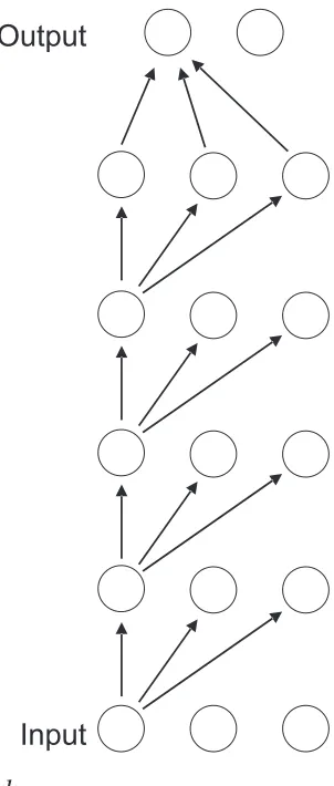
A multiple-layer feedforward network is generally illustrated as a stack of layers of “neurons” similar to what is shown in Figure 1-1 and Figure 1-2. The bottom layer is the input to the network, what would be referred to as the independent variables or predictors in traditional modeling literature. The layer above the input layer is the first hidden layer. Each neuron in this layer attains an activation that is computed by taking a weighted sum of the inputs, plus a bias, and then applying a nonlinear function. In the fully general case, each hidden neuron in this layer will have a different set of input weights.
If there is a second hidden layer, the activations of each of its neurons is computed by taking a weighted sum of the activations of the first hidden layer, plus a bias, and applying a nonlinear function. This process is repeated for as many hidden layers as desired.
In Figures 1-1 and 1-2, only a small subset of the connections is shown. Actually, every neuron in every layer feeds into every neuron in the next layer above.
Figure 1-1.
A shallow network
To be more specific, the activation of a hidden neuron, expressed as a function of the activations of the prior layer, is shown in Equation 1-1. In this equation, x = {x1, …, xK} is the vector of prior-layer activations, w = {w1, …, wK} is the vector of associated weights, and b is a bias term.
It’s often more convenient to consider the activation of an entire layer at once. In Equation 1-2, the weight matrix W has K columns, one for each neuron in the prior layer, and as many rows as there are neurons in the layer being computed. The bias and layer inputs are column vectors. The nonlinear activation function is applied element-wise to the vector.
a = f b +Wx
(
)
(1-2)There is one more way of expressing the computation of activations that is most convenient in some situations. The bias vector b can be a nuisance, so it can be absorbed into the weight matrix W by appending it as one more column at the right side. We then augment the x vector by appending 1 to it: x = {x1, …, xK, 1}. The equation for the layer’s activations then simplifies to the activation function operating on a simple matrix/vector multiplication.
a = f Wx
(
)
(1-3)Wide vs. Deep Nets
Prior to the development of neural networks, researchers generally relied on large doses of human intelligence when designing prediction and classification systems. One would measure variables of interest and then brainstorm ways of massaging these “raw” variables into new variables that (at least in the mind of the researcher) would make it easier for algorithms such as linear discriminant analysis to perform their job. For example, if the raw data were images expressed as arrays of gray-level pixels, one might apply edge detection algorithms or Fourier transforms to the raw image data and feed the results of these intermediate algorithms into a classifier.
The data-analysis world shook when neural networks, especially multiple-layer feedforward networks, came into being. Suddenly we had prediction and classification tools that, compared to earlier methods, relied to a much lesser degree on human-driven preprocessing. It became feasible to simply present an array of gray-level pixels to a neural network and watch it almost miraculously discover salient class features on its own.
habit was encouraged by several powerful forces. Theorems were proved showing that in very broad classes of problems, one or two hidden layers were sufficient to solve the problem. Also, attempts to train networks with more than two hidden layers almost always met with failure, making the decision of how many layers to use a moot point. According to the theorems of the day, you didn’t need deeper networks, and even if you did want more layers, you couldn’t train them anyway. So why bother trying?
The fly in the ointment was the fact that the original selling point of neural networks was that they supposedly modeled the workings of the brain. Unfortunately, it is well known that brains are far from shallow in their innermost computational structure (except for those of a few popular media personalities, but we won’t go there). And then new theoretical results began appearing that showed that for many important classes of problems, a network composed of numerous narrow layers would be more powerful than a wider, shallower network having the same number of neurons. In effect, although a shallow network might be sufficient to solve a problem, it would require enormous width to do so, while a deep network could solve the problem even though it may be very narrow. Deep networks proved enticing though still enormously challenging to implement.
The big breakthrough came in 2006 when Dr. Geoffrey Hinton et al. published the landmark paper “A Fast Learning Algorithm for Deep Belief Nets.” The algorithm described in this paper is generally not used for the training of convolutional nets, so we will not pursue it further here; for details, see Volume 1 of this series. Nevertheless, this algorithm is relevant to convolutional nets in that it allowed researchers to discover the enormous power of deep networks. We will see later that convolutional nets, because of their specialized structure, are much easier to train with conventional algorithms than fully general deep networks.
One of the most fascinating properties of deep belief nets, in their general as well as convolutional form, is their remarkable ability to generalize beyond the universe of training examples. This is likely because the output layer, rather than seeing the raw data, is seeing “universal” patterns in the raw data—patterns that due to their universality are likely to reappear in the general population.
Locally Connected Layers
As a general rule, the more optimizable weights we have in a neural network, the more problems we will have. All else being equal, training time goes up exponentially with the number of parameters being optimized. This is a major reason why, before the advent of specialized training algorithms and specialized network architectures, models having more than two hidden layers were practically unknown. Also, the more parameters we optimize, the more likely we are to overfit the model, treating noise in the training data as if it were authentic information.
When the input to the model is an image, it is often reasonable for neurons in a given layer to respond to only neurons in the prior layer that are nearby in the visual field. For example, a neuron in the upper-left corner of the first hidden layer may, by design, be sensitive to only pixels in the upper-left corner of the input image. It may be overkill to cause a neuron in the upper-left corner of the first hidden layer to react to pixels in the opposite corner of the input image.
By implementing this design feature, we tremendously reduce the number of optimizable weights in the model, yet we do not much reduce the total information capture. Even though the neurons in the first hidden layer may each respond to only nearby input neurons, taken as a whole the set of hidden neurons encapsulates information about the entire input image.
Figure 1-4.
Simple local connections
Rows, Columns, and Slices
Think about an input image. It may have multiple bands, such as RGB (red, green, blue). The image has a height (number of rows) and width (number of columns) that are the same for all three bands. In the context of convolutional nets, instead of speaking of bands, we may call them slices. In the same way, each hidden layer will occupy a volume described by a height, width, and depth (number of slices). Sometimes the height and width (the visual field) of a hidden layer will equal these dimensions of the prior layer, and sometimes they will be less. They will never be greater.
It can be helpful to think of a slice of a hidden layer as corresponding (roughly!) to a single hidden neuron in a conventional neural network. For example, in a conventional network we might have one hidden neuron responding to the sum of two inputs, and a different hidden neuron responding to the difference between these two inputs. In the same way, neurons in one slice may specialize in responding to the total input in the nearby visual field, while neurons in a different slice may specialize in detecting horizontal edges in the nearby visual field. This specialization may vary across the visual field, or it may be forced to be the same across the visual field. We will pursue this concept later.
To compute the activation of a single neuron in a hidden layer, we use an equation similar to Equation 1-1. However, it is considerably more complicated now because it involves only the prior-layer neurons that are nearby in the visual field and all prior-layer slices in this neighborhood. This is roughly expressed in Equation 1-5.
The equation for computing the activation of a single neuron in a locally connected hidden layer involves the following terms:
R : Row of neuron in layer being computed (we call this the current layer) C : Column of neuron in current layer
S : Slice of neuron in current layer
ARCS : Activation of the neuron (or input) being computed r : Row of neuron in prior layer (or input)
c : Column of neuron in prior layer (or input) s : Slice of neuron in prior layer (or input)
arcs : Activation of the prior-layer neuron (or input) at r, c, s
wRCSrcs : Weight associated with the prior-layer neuron (or input) at r, c, s when computing the activation of the neuron at RCS
ARCS= f b + w a
The developer defines what is meant by near in the model. Let NEARR be the number of prior-layer rows that, by design, are near the row being computed (which we call the current layer), and define NEARC similarly. Let NS be the number of slices in the prior layer, the depth of that layer. Then the number of weights involved in computing the activation of a neuron is NEARR * NEARS * NS plus one for the bias. As a convention in this book, I will often refer to this quantity (including the bias term) as nPriorWeights. Suppose there are NR rows in the current layer, as well as NC columns and NS slices. Then the total number of weights connecting the prior layer to the layer being computed is NR * NC * NS * nPriorWeights.
Astute readers will balk at one aspect of this computation. What about the edges of the prior layer, where on one or two sides there are no nearby prior-layer neurons? Great observation! Have patience…we will address this important issue soon.
Convolutional Layers
A few pages ago we mentioned that the pattern in which neurons in a slice specialize may be the same across the visual field, or it may vary. Neither is universally better than the other. If one is dealing with a variety of images, in which specific features do not have a pre-ordained position in the visual field, it probably makes sense for each layer to have a common specialization. For example, all neurons in one slice may respond to the local total brightness, while all neurons in a different slice may contrast the upper part of the local visual field with the lower part and hence be sensitive to a horizontal edge. On the other hand, if the input image is a prepositioned entity, such as a centered face or unknown military vehicle, then it probably makes sense to allow position-relative specialization. For example, neurons a little way in from the top left and top right may specialize in aspects of eye shape on a face.
If the application allows, there is one huge advantage to consistent specialization of a slice across the visual field. In this situation, the weight sets wRCSrcs are the same for all values of R and C, the position in the visual field of the neuron being computed. All neurons across the visual field of a given slice have the same weight set, meaning that the total number of weights connecting the prior layer to the current layer is now just
Such a layer is called a convolutional layer because each of its slices is based on the convolution of the prior layer’s activations with the nPriorWeights weight set that defines that slice’s specialization. (Convolution is a term from filtering theory. If you are unfamiliar with the term, no problem.) For clarity, the activation of a neuron in a convolutional layer is given by Equation 1-6.
ARCS= f b + w a
s r near R c nearC
Srcs rcs
å å
å
æ
è
çç ö
ø
÷÷ (1-6)
Half-Width and Padding
So far we have been vague about the meaning of near in the visual field. It’s time to be specific. Look back at Figure 1-4. We see that in both the vertical and horizontal directions, there are two neurons on either side of the center neuron. This distance is called the half-width of the filter. Although the vertical and horizontal half-widths are equal in this example, both being two, they need not be. However, the distance on either side (left-right and up-down from the center) are always equal; otherwise, the center would not be, um, the center. Denote the vertical and horizontal half-widths as HWV and HWH, respectively. Then Equation 1-7 gives the number of weights involved in computing the activation of a single neuron. Recall that NS is the number of slices in the prior layer. The +1 at the end is the bias term.
nPriorWeights = Ns
(
2HW +H 1) (
2HW +V 1)
+1 (1-7)We can now think about edge effect, the problem of a filter extending past the edge of the prior layer into undefined nothingness. We have two extreme options and perhaps a (rarely used) compromise between these two extremes.
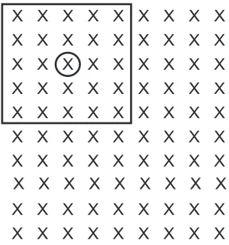
current layer will have its center in the prior layer at column HWH instead of the leftmost column. Thus, the intuitively nice alignment will be lost; each column of the current layer will be offset from the corresponding column of the prior layer by HWH. Similarly, we stop computation HWH columns before the right edge, and we also inset the top and bottom. This has the advantage of making use of all available information in an exact manner, but it has the disadvantage that rows and columns of the current layer are no longer aligned with rows and columns of the prior layer. This is usually of little or no practical consequence, but it is troubling on a gut level. See Figure 1-5.
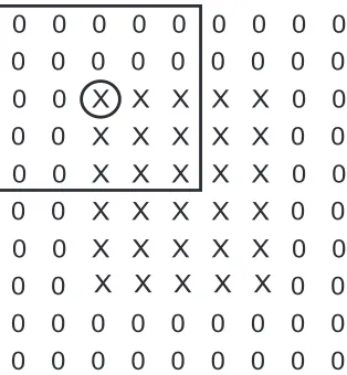
2. Pad the prior layer with HWH columns of zeros on the left and right sides, and HWV rows of zeros on the top and bottom, to provide “defined” values for the outside-the- visual-field neurons when we place the center of the filter on the edge. This lets us preserve layer-to-layer alignment of neurons in the visual field, which gives most developers a warm, fuzzy feeling and hence is common. It also has an advantage in many CUDA implementations, which I’ll touch on in a moment. But it’s fraught with danger, as we’ll discuss in a moment. See Figure 1-6.
In Figures 1-5 and 1-6, the square box outlines the neurons in the visual field of the prior layer that impact the activation of the top-left neuron in a slice of the current layer. The center of the box is circled. The top-left X in these figures is the top-left neuron in the prior layer. Figure 1-5 shows that the top-left neuron in the slice being computed is centered in the visual field two neurons in and two neurons down from the prior layer’s top left. In Figure 1-6, we see that the top-left neuron in the slice being computed also corresponds to the top-left neuron in the prior layer because those zeros let the filter extend past the edge.
But make no mistake, those zeros have an impact. It’s easy to dismiss them as “nothing” numbers. This feeling is made all the more acceptable because when we program this, we simply avoid adding in the components of Equation 1-5 that
correspond to the overhang. Hey, if you don’t add them in, they can’t do any harm, right? Those weights are just ignored.
Unfortunately, zero is not nothing; it is an honest-to-goodness number. For example, suppose the prior layer is an input image, scaled 0–255. Then zero is pure black! If the weight set computes an average luminance, these zeros will pull the average well down into gray even if the legitimate values are bright. If the weight set detects edges and the legitimate values are bright, a profound edge will be flagged here. For this reason, I am cautious about zero padding. On the other hand, it appears to be more or less standard. You pays your money, and you take your choice.
function, the effect of zero padding would be even more severe. Also note that in my CONVNET program, I rescale input images to minus one through one rather than the more common 0–255. This lessens the impact of zero padding.
I should add that full zero padding can be advantageous in many CUDA
implementations. This will be discussed in detail later when we explore CUDA code, but the idea is that certain numbers of hidden neurons, such as multiples of 32, speed operation by making memory accesses more efficient. On the other hand, lack of full zero padding impacts only the size of the visual field, not the depth, and good CUDA implementations can compensate for shrinking visual fields by handling the depth dimension properly.
Note that one is not bound to employ one of these two extreme options. It is perfectly legitimate to compromise and pad with fewer than HWH columns of zeros on the left and right, and HWV rows of zeros on the top and bottom. Nobody seems to do it, but you needn’t let that stop you.
Striding and a Useful Formula
A common general principle of neural network design is that the size of hidden layers decreases as you move from input toward output. Of course, we can (and usually do) decrease the depth (number of slices) of successive layers. But effective information compression is also obtained by decreasing the size of the visual field (rows and
columns) in successive layers. If we pad with half-width zeros as in option 2 in the prior section, the size of the visual field remains constant. And even if we do not pad, the visual field only slightly decreases. There is a more direct approach: striding.
It should be emphasized that the modern tendency is to avoid striding and use pooling to reduce the visual field. That topic will be discussed later in the chapter. However, because striding does have a place in our toolbox, we’ll cover it now.
We now present a simple formula for the number of rows/columns in the current layer, given the size of the prior layer and the size of the filter, the amount of zero padding, and the stride. No identification of vertical or horizontal is needed, as this formula applies to each dimension. The following definitions for the terms of the formula in Equation 1-8 apply:
W: Width/height of the prior layer
F: Width/height of the filter; two times half-width, plus one
P: Padding rows/columns appended to each edge; less than or equal to half-width S: Stride
C: Width/height of the current layer
C = W
(
-F + P2)
/S+1 (1-8)There is widespread belief that the division by the stride must be exact; if the numerator is not a multiple of the stride, the layer is somehow invalid. A brief Internet search shows this belief to be ubiquitous. But it’s not really true. There are two things that make this belief appealing.
• If the division is not exact, the alignment of the current layer with the prior layer will not be symmetric; the current layer may be inset from the prior layer by different amounts on the right and left, or top and bottom. However, I do not see any reason in any application why this lack of symmetry would be a problem. If this is a problem in your application, then select your parameters in such a way as to make the division exact. But it’s silly for the padding to exceed the half-width, and the filter size may be important and not amenable to change. This can make it difficult to produce perfect division.
Pooling Layers
The prior section discussed striding, a means of reducing the size of the visual field when progressing from one layer to the next. Although this method was popular for some time and is still occasionally useful, it has recently been supplanted by the use of a pooling layer. In particular, the stride of a locally connected or convolutional layer is generally kept at one so that the visual field is left unchanged (if full padding) or only slightly reduced (if less than full padding). Then, a layer whose sole purpose is to reduce the visual field is employed.
Pooling layers are similar to locally connected/convolutional layers in that they move a rectangular window across the prior layer, applying a function to the activation values in each window to compute the activation of a single neuron in the current layer. But the biggest difference is that pooling layers are not trainable. Their function, which maps window values in the prior layer to an activation in the current layer, is fixed in advance.
There are three other differences. Padding is generally not used; it is avoided in this book, as I believe the distortion introduced by padding a pooling layer is too risky. Also, filter widths can be even; they do not take the form 2*HalfWidth+1. The implication is that pooling destroys layer-to-layer alignment.
Finally, the pooling function that maps the prior layer to the current layer is applied separately to each slice. The locally connected/convolutional layers discussed in the previous few sections look at all prior-layer slices simultaneously. So, for example, if we have a five-by-five filter operating on a prior layer that has ten slices, a total of 5*5*10=250 activations in the prior layer take part in computing the activation of a neuron in the current layer. But in a pooling layer, there are as many slices as in the prior layer, and each layer is computed independently. So, using these same numbers, each of the ten neurons in the current layer occupying the same position in the visual field would be computed from 25 prior-layer activations in the corresponding slice. We map first slice to first slice, second slice to second slice, and so forth.
Pooling Types
The most popular type of pooling as of this writing is max pooling. This mapping function chooses the neuron in the prior layer’s window, which has maximum activation. Much experience indicates that this is more effective than average pooling.
One small but annoying disadvantage of max pooling is that it is not differentiable everywhere. At the activation levels where the choice transitions from one neuron to another, the derivative of the performance criterion with respect to a particular weight goes to zero on the neuron suddenly losing the contest and jumps away from zero on the winner. This slightly impedes some optimization algorithms, and it makes numerical verification of gradient computations a bit dicey. But in practice, these problems do not seem to be overly serious, so we put up with them.
Other pooling functions are appearing. Different norms can be used, and some even more exotic functions have been proposed. None of these alternatives is discussed in this book.
The Output Layer
This book, as well as the CONVNET program, follows the simple convention that the output layer contains one neuron for each class. Each of these neurons is fully connected to all neurons in the prior layer. Because the concept of visual field makes no sense in the concept of output-layer classes, this layer by definition is organized as a single row and column (the “visual field” is one pixel) with a depth (number of slices) equal to the number of classes. The exact organizational layout is not vital, but this layout proves to simplify programming and mathematical derivations.
SoftMax Outputs
In these more enlightened times, we can “soften” the selection process, making the predicted outputs resemble probabilities. This is extremely useful, not just because it’s nice to be able to talk about the predicted probability of each class (even though in many applications this interpretation is excessively optimistic!) but also for an even more important reason. These SoftMax outputs make the model far more robust against outliers in the training and test data. This vital topic is discussed in detail in Volume 1 of this series, so it will be glossed over here. But we do need to review the relevant equations that we will program.
We know that the activation of a single hidden neuron is computed as a nonlinear function of a weighted average of prior-layer activations (plus a bias term). For the output neurons we drop the nonlinear function and speak only of the weighted average (plus bias). This quantity is called the logit of the neuron being computed. This is shown in Equation 1-9 for output neuron k. In this equation, x = {x1, x2, …} is the vector of activations of the final hidden layer, w = {wk1, wk2, …} is the vector of associated weights, and bk is a bias term. In other words, the logit of an output neuron is computed exactly like we compute the activation of a hidden-layer neuron, except that we do not apply the nonlinear activation function.
logit = b +k k w x i
ki i
å
(1-9)Once we have the logit of every output neuron, computing the SoftMax output values, which can roughly be thought of as probabilities of class membership, is done with Equation 1-10. This equation assumes that there are K output neurons (classes). It should be obvious that these output activations are non-negative and sum to one.
p y = k = e
Any set of model parameters defines, by means of the equations just shown, the probability of each possible class given an observed case. Our training set is assumed to be random draws from a population, each of which provides an input vector and a true class. If we were to consider a given set of model parameters as defining the true model, we could compute (in a sense best left undiscussed here) the probability of obtaining the set of training cases that were actually observed. So we find that set of parameters that maximizes this probability. In other words, we seek the model that provides the maximum likelihood of having obtained our training set in these random draws from the population.
In our particular application, the likelihood of a case is just the probability given by the model for the class to which that case belongs. We want a criterion that is summable across the training set, so instead of considering the likelihood, which is multiplicative, we will use the log likelihood as our criterion. This way we can compute the criterion for the entire training set by summing the values for the individual cases in the training set.
Also, to conform to more general forms of the log likelihood function that you may encounter in more advanced texts, as well as to conform to the expression of the derivative that will soon be discussed, we express the log likelihood of a case in a more complex manner. For a given training case, define tk as 1.0 if this case is a member of class k, and 0.0 otherwise. Also define pk as the SoftMax activation of output neuron k, as given by Equation 1-10. Then, for our single training case, the log of the likelihood corresponding to the model’s parameters is given by Equation 1-11. This equation is called the cross entropy, and interested readers might want to look up this term for some fascinating insights.
Observe that in the summation over classes, every term is zero except the term corresponding to the correct class. Thus, the log likelihood is just the log of the model’s computed probability for the correct class of the case. Here are some observations about the log likelihood:
• Because p is less than one, the log likelihood is always negative.
• If the model is nearly perfect, meaning that the computed probability of the correct class is nearly 1.0 for every case, the log likelihood will approach zero, its maximum possible value.
We will soon discuss gradient computation, at which time we will need the derivative of the log likelihood. Without going through the considerable number of steps, we state that this derivative of Equation 1-11 for a case is given by Equation 1-12.
d 
Developers with experience in computing the gradient of traditional neural networks will be amazed to see that, except for a factor of two, the delta for a SoftMax output layer and maximum likelihood optimization is identical to that for a linear output layer and mean-squared-error optimization. This means that traditional predictive model gradient algorithms can be used for SoftMax classification with only trivial modification. Nonetheless, we will summarize gradient computation in the next section.
Back Propagation of Errors for the Gradient
The fundamental goal of supervised training can be summarized simply: find a set of parameters (weights and biases as in Equation 1-2) such that, given an input to the neural network, the output of the network is as close as possible to the desired output. To find such parameters, we must have a performance criterion that rigorously defines the concept of “close.” We then find parameters that optimize this criterion.
Suppose we have K output neurons numbered 1 through K. For a given training case, let tk be the true value for this case, the value that we hope the network will produce, and let pk be the output actually obtained. Then the log likelihood for this single case is given by Equation 1-11. To compute the log likelihood for the entire training set, sum this quantity for all cases. To keep this quantity to “reasonable” values, most people (including me) divide this sum by the number of cases and the number of classes. If there are N training cases, this performance criterion is given by Equation 1-13.
Supervised training of a multiple-layer feedforward network amounts to finding the weights and bias terms that maximize Equation 1-13 (or minimize its negative, which is what we really do). In any numerical minimization algorithm, it is of great benefit to be able to efficiently compute the gradient, the partial derivatives of the criterion being minimized with respect to each individual parameter. Luckily, this is quite easy in this application. We just start at the output layer and work backward, repeatedly invoking the chain rule of differentiation.
The activation of output neuron k is given by Equation 1-10. Neural net aficionados use the Greek letter delta to designate the derivative of the performance criterion with respect to the net input coming into a neuron; in the current context this is output neuron k, and its delta is given by Equation 1-12.
In other words, this neuron is receiving a weighted sum of activations from all neurons in the prior layer, and from Equation 1-12 we know the derivative of the log likelihood criterion with respect to this weighted sum.
How can we compute the derivative of the criterion with respect to the weight from neuron i in the prior layer? The simple chain rule tells us that this is the product of the derivative in Equation 1-12 times the derivative of the net input (the weighted sum coming into this output neuron) with respect to this weight.
This latter term is trivial. The contribution to the weighted sum from neuron i in the prior layer is just the activation of that neuron times the weight connecting it to the output neuron k. We shall designate this output weight as wkiO. So the derivative of that weighted sum with respect to wkiO is just the activation of neuron i. This leads us to the formula for the partial derivatives of the criterion with respect to the weights connecting the last hidden layer to the output layer. In Equation 1-14 we use the superscript M on a to indicate that it is the activation of a neuron in hidden layer M, where there are M hidden layers numbered from 1 through M.
As before, the former term here is trivial: just the activation of the prior neuron feeding through this weight. It’s the latter that’s messy.
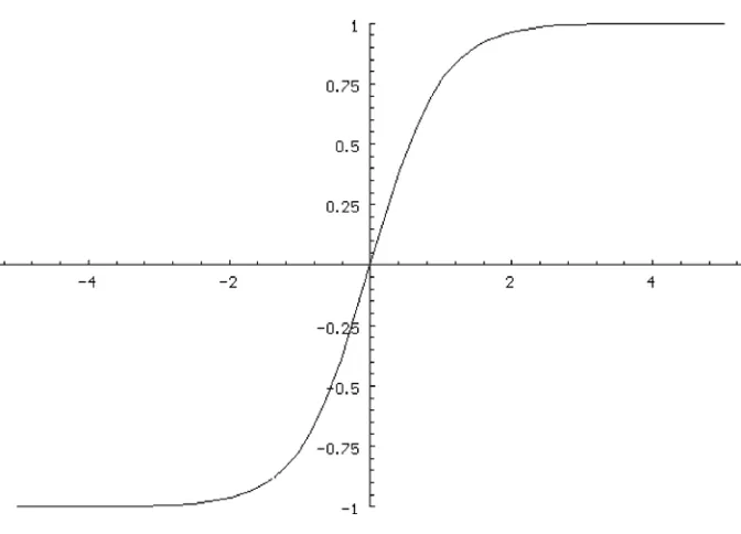
The first complication is that the hidden neurons are nonlinear. In particular, the function that maps the net input of a hidden neuron to its activation is the hyperbolic tangent function shown in Equation 1-4. So the chain rule tells us that the derivative of the criterion with respect to the net input is the derivative of the criterion with respect to the output times the derivative of the output with respect to the input. Luckily, the derivative of the hyperbolic tangent function f (a) is simple, as shown in Equation 1-15.
f a =¢
( )
1- f2( )
a (1-15)The remaining term is more complicated because the output of a neuron in a hidden layer feeds into every neuron in the next layer and thus impacts the criterion through every one of those paths. Recall that δkO is the derivative of the criterion with respect to the weighted sum coming into output neuron k. The contribution to this weighted sum going into output neuron k from neuron i in the prior layer M is the activation of hidden neuron i times the weight connecting it to output neuron k. So the impact on the derivative of the criterion from the activation of neuron i that goes through this path is δkO times the connecting weight. Since neuron i impacts the error through all output neurons, we must sum these contributions, as shown in Equation 1-16.
Pant pant. We are almost there. Our goal, the partial derivative of the criterion with respect to the weight connecting a neuron in hidden layer M−1 to a neuron in hidden layer M is the product of the three terms that we have already presented.
• The derivative of the net input to the neuron in hidden layer M with respect to the weight in which we are interested
• The derivative of the output of this neuron with respect to its net input (the derivative of its nonlinear activation function)
The derivative of the criterion with respect to wijM (the weight connecting neuron j in layer M−1 to neuron i in layer M) is the product of these three terms. The product of the second and third of these terms is given by Equation 1-17, with f ′(.) being given by Equation 1-15. The multiplication is completed in Equation 1-18.
di ¢ d
There is no need to derive the equations for partial derivatives of weights in hidden layers prior to the last hidden layer, as the equations are the same, just pushed back one layer at a time by successive application of the chain rule. In particular, for some hidden layer m<M, we have Equation 1-19 for the partial derivative of the criterion with respect to the weighted sum coming into neuron i in layer m. Equation 1-20 then provides the partial derivative of the criterion with respect to the weight connecting neuron j in hidden layer m−1 to neuron i in hidden layer m. In this case, there are K neurons in hidden layer m+1.
That was a long haul, especially for those for whom math is not pleasant. So as an aid to those who are mainly interested in programming, here is a more concise summary of the procedure for computing the gradient:
1. Allocate two scratch vectors, this_delta[] and prior_delta[]. These must be as long as the maximum number of hidden neurons in any layer, as well as the number of classes (output neurons).
2. Compute activations for all hidden layers and the output layer.
3. Use Equation 1-12 to compute the output deltas. Put these in this_delta.
5. Designate the last hidden layer as the “current” layer, which makes the output layer the “next” layer.
6. This is the beginning of the main loop that moves backward through the network, from the last hidden layer to the first. At this time, this_delta[k] contains the derivative of the criterion with respect to the input (post-weight) to neuron k in the next layer.
7. Backpropagate delta. To get the contribution of that neuron k from neuron i in the current layer, the layer whose gradient is currently being computed, we multiply delta[k] by the weight connecting current-layer neuron i to next-layer neuron k. This gives us the part of the total derivative due to the output of neuron i in the current layer going through neuron k in the next layer. But the output of neuron i impacts the criterion derivative through all neurons in the next layer. Thus, we must sum these parts across all neurons (values of k) in the next layer. To get the derivative of the criterion with respect to the input to neuron i, we multiply this sum by the derivative of neuron i’s activation function. This is Equation 1-19, or Equation 1-17 if this is the last hidden layer. The arguments for this equation are in this_delta, and we put the results in prior_delta.
8. Move the contents of prior_delta to this_delta.
9. To get the derivative of the criterion with respect to a weight coming into neuron i, we multiply delta by the input coming through this weight (the output of the prior layer’s neuron). This is Equation 1-20, or Equation 1-18 if this is the last hidden layer. If there are more hidden layers to process, go to step 6.
Programming Algorithms
The source code that can be downloaded for free from my web site contains four large source files that handle the vast majority of the computation involved in propagating activations and backpropagating deltas for all layer types involved in convolutional nets.
• MOD_NO_THR.CPP: Nonthreaded versions of all routines. These are not used in the CONVNET program, but they are the routines listed and discussed in this book. Because they are not designed for threaded use, they are somewhat simpler than the threaded versions. In this way, the focus of discussion can be on the algorithms themselves, avoiding the complexities of threading.
• MOD_THR.CPP: Threaded versions of all routines. The last section of this chapter will explore how they differ from the nonthreaded versions and how they are incorporated into a fully multithreaded program.
• MOD_CUDA.CPP: Host routines that call the CUDA routines and coordinate all CUDA-based computation.
• MOD_CUDA.cu: All CUDA source code, as well as their host-code wrappers. Note that cu is lowercase. For some bizarre reason, Visual Studio has problems when it is in uppercase. Go figure.
Here is the order in which routines will be presented in this chapter: 1. Extract of Model declaration, showing key declarations
2. Extract of Model constructor, showing how architecture is built 3. trial_no_thr(), externally callable routine that computes all
activations
5. trial_error_no_thr(), externally callable routine to compute criterion
6. grad_no_thr(), externally callable routine to compute gradient 7. Gradient routines for each layer type; called from grad_no_thr() 8. Backprop routines for each layer type; called from gradient
routines
9. Discussion of threading the algorithms
Model Declarations
The complete set of model declarations can be found in the file CLASSES.H. However, most of them are irrelevant to the discussion of the activation and gradient algorithms, so they are not printed in the text.
Also, there are a handful of variables used so extensively that I (please forgive me!) made them global. They are as follows:
int n_pred; // Number of predictors present (input rows*cols*bands) int n_classes; // Number of classes
int n_db_cols; // Size of a case in the database = n_pred + n_classes int n_cases; // Number of cases (rows) in database
double *database; // They are here, variables changing fastest
int IMAGE_rows; // Input number of rows int IMAGE_cols; // and columns
int IMAGE_bands; // Its number of bands
Here are the important Model class declarations for convenient reference. Note that some duplicate globals. The declarations that are arrays have separate values for each layer.
int n_pred; // Number of predictors present (input grid size; rows*cols*bands) int n_classes; // Number of classes
int n_layers; // Number of hidden layers (does not include input or output) int layer_type[]; // Each entry is type of layer
int nhid[]; // Number of neurons in this layer = height times width times depth int HalfWidH[]; // Horizontal half width looking back to prior layer
int HalfWidV[]; // And vertical
int padH[]; // Horizontal padding, must not exceed half width int padV[]; // And vertical
int strideH[]; // Horizontal stride int strideV[]; // And vertical
int PoolWidH[]; // Horizontal pooling width looking back to prior layer int PoolWidV[]; // And vertical
int n_prior_weights[]; // N of inputs per neuron (including bias) from prior layer // = prior depth * (2*HalfWidH+1) * (2*HalfWidV+1) + 1 // A CONV layer has this many weights per slice // A LOCAL layer has this times its nhid
int n_hid_weights; // Total number of all hidden weights; includes bias int n_all_weights; // As above, but also includes output layer weights
int max_any_layer; // Max n of neurons in any layer, including input and output double *weights; // All ‘n_all_weights’ weights, including final weights, are here double *layer_weights[]; // Pointers to each layer’s weights in ‘weight’ vector
double *gradient; // ‘n_all_weights’ gradient, aligned with weights double *layer_gradient[]; // Pointers to each layer’s gradient in ‘gradient’ vector double *activity[]; // Activity vector for each layer
double *this_delta; // Scratch vector for gradient computation double *prior_delta; // Ditto
double output[]; // SoftMax activation for each class
int *poolmax_id[]; // Used only for POOLMAX layer; saves from forward pass ID
Order of Weights and Gradient
The weights for layer i begin at layer_weights[i]. Similarly, the gradient (which aligns element by element with the corresponding weights) for layer i begin at layer_gradient[i].
Two general ordering rules govern all layer types.
For a fully connected layer, these two rules clearly describe the situation. First we have the n_prior_weights weights connecting the prior layer to the first hidden neuron, with the bias last. Within that vector, the prior layer’s width changes fastest, then the height, and finally the depth slowest. After this, we have a similar vector for the second neuron in the current layer, and so forth. Recall that in a fully connected layer, the height and width are both one, with neurons strung out along the depth.
For other layer types, the order is slightly more complex and will be described as each activation routine is presented.
Initializations in the Model Constructor
Most of the code in the Model constructor is mundane and not worth listing in this text. You can see the full module in MODEL.CPP. However, some of this code reinforces discussions in the prior chapter and so is presented here.
In the loop shown next, we compute n_prior_weights in three steps for locally connected and convolutional layers. First we set it equal to the size of the moving- window filter, the number of weights in the filter. Then we multiply this by the number of slices in the prior layer because the filter is applied to all prior-layer slices simultaneously. Finally, we add 1 to include the bias term. Also in this loop we use Equation 1-8 to compute the size of the visual field.
for (i=0; i<n_layers; i++) {
nfH = 2 * HalfWidH[i] + 1; // Filter width nfV = 2 * HalfWidV[i] + 1;
if (layer_type[i] == TYPE_LOCAL || layer_type[i] == TYPE_CONV) {
n_prior_weights[i] = nfH * nfV; // Inputs, soon including bias, to neurons in layer if (i == 0) {
height[i] = (IMAGE_rows - nfV + 2 * padV[i]) / strideV[i] + 1; width[i] = (IMAGE_cols - nfH + 2 * padH[i]) / strideH[i] + 1; n_prior_weights[i] *= IMAGE_bands;
} else {
height[i] = (height[i-1] - nfV + 2 * padV[i]) / strideV[i] + 1; width[i] = (width[i-1] - nfH + 2 * padH[i]) / strideH[i] + 1; n_prior_weights[i] *= depth[i-1];
}
By common convention, a fully connected layer is implemented as a one-pixel visual field, with a slice for each neuron. It has a weight from every prior-layer activation, plus the bias term.
else if (layer_type[i] == TYPE_FC) { height[i] = width[i] = 1;
if (i == 0)
n_prior_weights[i] = n_pred + 1; else
n_prior_weights[i] = nhid[i-1] + 1; }
Pooling layers also have their visual field size defined by Equation 1-8. They align slice by slice with the prior layer, each processed independently, so a pooling layer has the same number of slices as the prior layer. Padding is never used (by me anyway) for pooling layers. Pooling layers are a fixed function, with no trainable weights, so n_prior_ weights is zero. Finally, the number of hidden neurons in this layer, regardless of type, is the product of the dimensions.
else if (layer_type[i] == TYPE_POOLAVG || layer_type[i] == TYPE_POOLMAX) { if (i == 0) {
height[i] = (IMAGE_rows - PoolWidV[i]) / strideV[i] + 1; width[i] = (IMAGE_cols - PoolWidH[i]) / strideH[i] + 1; depth[i] = IMAGE_bands;
} else {
height[i] = (height[i-1] - PoolWidV[i]) / strideV[i] + 1; width[i] = (width[i-1] - PoolWidH[i]) / strideH[i] + 1; depth[i] = depth[i-1];
}
n_prior_weights[i] = 0; }
The previous code handles the hidden layers. We do the output layer, which is always fully connected, in the following code. We don’t need to worry about the height, width, and depth because they will never be referenced in subsequent code that processes the output layer.
if (n_layers == 0)
n_prior_weights[n_layers] = n_pred + 1; // Output layer, always fully connected else
n_prior_weights[n_layers] = nhid[n_layers-1] + 1;
Lastly, we compute the total number of weights in all hidden layers, not including the output layer. We also need the maximum size of any layer, input, hidden, or output. These will be used for memory allocation, not shown here. This code is presented only to reinforce architectural issues in the model.
The most important fact here is that locally connected and fully connected layers have a number of weights equal to n_prior_weights times the number of hidden neurons in the layer because each hidden neuron has its own set of weights. But a convolutional layer has a number of weights equal to n_prior_weights times the depth of this layer because every neuron in the visual field of a given slice shares the same set of weights.
max_any_layer = n_pred; // Input layer is included in max if (n_classes > max_any_layer)
max_any_layer = n_classes; // Output layer is included in max
n_hid_weights = 0;
for (ilayer=0; ilayer<n_layers; ilayer++) { // For each of the hidden layers if (nhid[ilayer] > max_any_layer)
max_any_layer = nhid[ilayer];
if (layer_type[ilayer] == TYPE_FC || layer_type[ilayer] == TYPE_LOCAL) n_hid_weights += nhid[ilayer] * n_prior_weights[ilayer];
else if (layer_type[ilayer] == TYPE_CONV)
n_hid_weights += depth[ilayer] * n_prior_weights[ilayer];
else if (layer_type[i] == TYPE_POOLAVG || layer_type[i] == TYPE_POOLMAX) n_hid_weights += 0; // Just for clarity; pooling has no trainable weights } // For ilayer (each hidden layer)
Finding All Activations
The routine trial_no_thr() can be called from elsewhere. It does a forward pass to compute all activations in the model. None of the nitty-gritty calculations appears here; the routine simply calls the appropriate specialist for each layer.
void Model::trial_no_thr (double *input) {
int i, ilayer; double sum;
for (ilayer=0; ilayer<n_layers; ilayer++) { // These do not include output layer if (layer_type[ilayer] == TYPE_LOCAL)
activity_local_no_thr (ilayer, input); else if (layer_type[ilayer] == TYPE_CONV) activity_conv_no_thr (ilayer, input); else if (layer_type[ilayer] == TYPE_FC) activity_fc_no_thr (ilayer, input, 1);
else if (layer_type[ilayer] == TYPE_POOLAVG || layer_type[ilayer] == TYPE_POOLMAX) activity_pool_no_thr (ilayer, input);
}
activity_fc_no_thr (n_layers, input, 0); // Output layer
// Classifier is always SoftMax. Use Equation 1-10 on Page 16.
sum = 1.e-60; // Denominator below must never be zero for (i=0; i<n_classes; i++) {
if (output[i] < 300.0) // Be safe against rare but deadly problem output[i] = exp (output[i]);
else
output[i] = exp (300.0); sum += output[i]; }
Activating a Fully Connected Layer
Computing the activation of a fully connected layer is relatively easy because every neuron in the layer is connected to every neuron in the prior layer. We do not have to worry about the position of a moving window or whether we are past the edge of the prior layer, or striding, and so forth. These considerations can be surprisingly complicated to implement efficiently. Thus, we begin with this easy routine.
One potential source of confusion is the input parameter. This is not the input to the layer being computed; if this layer is past the first hidden layer, the input to this layer will be fetched directly from the activity vector of the prior hidden layer. Rather, this is the input to the model, and it is used only if this is the first layer after the input.
void Model::activity_fc_no_thr (int ilayer, double *input, int nonlin) {
int iin, iout, nin, nout;
double sum, *wtptr, *inptr, *outptr;
wtptr = layer_weights[ilayer]; // Weights for this layer
if (ilayer == 0) { // The ‘prior layer’ is the input vector
nin = n_pred; // This many elements in the vector inptr = input; // They are here
}
else { // The prior layer is a hidden layer nin = nhid[ilayer-1]; // It has this many neurons inptr = activity[ilayer-1]; // Prior layer’s activations }
if (ilayer == n_layers) { // If this is the output layer
nout = n_classes; // There is one output neuron for each class outptr = output; // Outputs go here
}
else { // This is a hidden layer
nout = nhid[ilayer]; // We must compute this many activations outptr = activity[ilayer]; // And put them here
for (iout=0; iout<nout; iout++) { // Compute each activation
sum = 0.0;
for (iin=0; iin<nin; iin++) // Equation 1-1 on Page 3 sum += inptr[iin] * *wtptr++;
sum += *wtptr++; // Bias
if (nonlin) { // Hidden layers are nonlinear; output is not sum = exp (2.0 * sum); // Hyperbolic tangent function
sum = (sum - 1.0) / (sum + 1.0); // Equation 1-4 on Page 3 }
outptr[iout] = sum; }
}
Activating a Locally Connected Layer
First, we must be clear on how the weights that connect the prior layer to this locally connected layer are ordered. They can best be visualized as they would be processed in a set of nested loops:
Current layer depth Current layer height
Current layer width Prior layer depth
Prior layer height Prior layer width Bias
The depth dimension of the neuron being computed changes slowest, then the height, and finally the width. At the width point (three levels in), we are looking at the weights for computing a single neuron in this layer. We have the weights that connect it to the prior layer, in the order shown. After these prior-layer weights appear, we have the single bias term.
void Model::activity_local_no_thr (int ilayer, double *input) {
int k, in_row, in_rows, in_col, in_cols, in_slice, in_slices, iheight, iwidth, idepth; int rstart, rstop, cstart, cstop;
double sum, *wtptr, *inptr, *outptr, x;
if (ilayer == 0) { // This is the first layer after the input in_rows = IMAGE_rows;
in_cols = IMAGE_cols; in_slices = IMAGE_bands;
inptr = input; // Input to this layer is the model’s input image }
else { // The prior layer is a hidden layer in_rows = height[ilayer-1];
in_cols = width[ilayer-1]; in_slices = depth[ilayer-1];
inptr = activity[ilayer-1]; // Input to this layer is the prior layer’s activations }
wtptr = layer_weights[ilayer]; // Weights for this layer, order as described above outptr = activity[ilayer]; // We put the computed activations here
k = 0; // This will index the computed activations in outptr for (idepth=0; idepth<depth[ilayer]; idepth++) {
for (iheight=0; iheight<height[ilayer]; iheight++) { for (iwidth=0; iwidth<width[ilayer]; iwidth++) {
// Compute activation of this layer’s neuron at (idepth, iheight, iwidth)
We can now compute the inclusive starting and stopping rows and columns of the rectangle in the prior layer, which contributes to the activation of the neuron in the current layer. We start at -Pad, advance by Stride as the current layer advances, and end at twice the HalfWidth.
sum = 0.0; // Will sum the filter here
// Center of first filter is at HalfWidth-Pad; filter begins at -Pad. rstart = strideV[ilayer] * iheight - padV[ilayer];
rstop = rstart + 2 * HalfWidV[ilayer];
cstart = strideH[ilayer] * iwidth - padH[ilayer]; cstop = cstart + 2 * HalfWidH[ilayer];
We are now ready to compute the weighted sum of the prior layer’s activations in the rectangle. Recall that the filter sums across all slices in the prior layer. Astute readers, and even not-so-astute readers, will notice a small but significant inefficiency in how I program the logic for handling zero padding outside the edges of the prior layer. The row test can be done outside the column loop since its result will be the same for all columns! However, I deliberately did it this way here for clarity. It should be trivial for interested readers to fix this. It is also possible to limit the rectangle bounds in advance so that no test is necessary. But that complicates weight addressing a lot and likely would be no faster.
for (in_slice=0; in_slice<in_slices; in_slice++) { for (in_row=rstart; in_row<=rstop; in_row++) { for (in_col=cstart; in_col<=cstop; in_col++) {
// This logic is a bit inefficient
if (in_row >= 0 && in_row < in_rows && in_col >= 0 && in_col < in_cols) x = inptr[(in_slice*in_rows+in_row)*in_cols+in_col];
else // We are outside the visual field, in the zero padded area x = 0.0;
sum += x * *wtptr++; // Equation 1-1 on Page 3
sum += *wtptr++; // Bias in Equation 1-1
sum = exp (2.0 * sum); // Hyperbolic tangent activation function sum = (sum - 1.0) / (sum + 1.0); // Equation 1-4 on Page 3
outptr[k++] = sum; } // For iwidth } // For iheight } // For idepth }
Activating a Convolutional Layer
The code for activating a convolutional layer is almost identical to that for activating a locally connected layer. This is because the only difference between the two is that in a convolutional layer, for a given slice, all neurons in the visual field share the same set of weights. In a more general locally connected layer, the neurons all have their own weight sets.
For this reason, it’s a borderline waste of trees to reproduce the code here. Still, I think it’s instructive to compare them. I suggest that you flip pages back and forth, comparing the two algorithms. I’ll jump right in, stopping only to point out the salient differences.
First, let’s again consider how the weights that connect the prior layer to this convolutional layer are ordered. This is identical to the locally connected ordering, except that the height and width are omitted because the weights are the same for every neuron in the visual field.
Current layer depth Prior layer depth
Prior layer height Prior layer width Bias
void Model::activity_conv_no_thr (int ilayer, double *input) {
int k, in_row, in_rows, in_col, in_cols, in_slice, in_slices, iheight, iwidth, idepth; int rstart, rstop, cstart, cstop;