Individual base model of predator-prey system shows
predator dominant dynamics
Yoshinori Takahara *
Department of Geology,Uni6ersity of California at Da6is,Da6is,CA95616USA Received 5 April 2000; received in revised form 8 August 2000; accepted 21 August 2000
Abstract
Individual base model of predator-prey system is constructed. Both predator and prey species have age structure and cohorts of early reproductive age have competitive advantage. The model has linear functional response in predation behavior and includes the effect of interference among predators and delay of population growth from resource intake, not by functional response but by calculation procedure. Each foraging action is calculated successively and surplus or scarce of acquired resources is interpreted into population size through individual birth and death. This model shows that biomass of prey killed by predator is dependent on demand of predator and that heterogeneity in predator population is essential in persistency and stability of predator-prey system. Heterogeneity of predator makes predator individuals of less competing ability die rapidly. Rapid death of weak individuals causes rapid decrease of total demand of predator and that makes enough room for survived predators. Therefore, the biomass of killed prey is dependent on predator’s demand. As young or infant population of predator are the more vulnerable to shortage of prey, and when many of them cannot survive to reproductive age, they can stabilize the system by wasting excessive prey with only temporal numerical increase of predator population. © 2000 Elsevier Science Ireland Ltd. All rights reserved.
Keywords:Individual base model; Inside observer; Predator-prey system; Predator-dependent; Prey-dependent; Ratio-dependent www.elsevier.com/locate/biosystems
1. Introduction
Mass action models based upon Lotka – Volterra equations (Lotka, 1925; Volterra, 1926) have been adopted in many works as a model for predator-prey system. Most simple models of
these conventional ones assume that all individu-als within each species are identical in trophic dynamics and that predator’s feeding rate (the functional response) depends on prey density alone. These models make a prediction known as the paradox of enrichment, which was termed by Rosenzweig (1971). The prediction is that enrich-ment of the prey population by increased prey carrying capacity will result in limit cycle oscilla-tion that grow rapidly in amplitude with further enrichment. May (1972), Gilpin (1972, 1975) and Yodzis and Innis (1992) modeled it.
* Present address: Department of Bioengineering, Nagaoka University of Technology, Nagaoka, Niigata 940-2188, Japan. Tel:+81-258-479416; fax:+81-258-479400.
E-mail address:[email protected] (Y. Takahara).
Both field data and laboratory experiments provide little support for this prediction. Most natural populations seem to lack such regular fluctuations (Pimm, 1991). On the other hand, simple experiments in a microcosm show two species predator-prey system in a closed system can hardly persist (Gause, 1934) as Gilpin (1975) and Yodzis and Innis (1992) questioned whether such cycling systems as had sensitivity of ampli-tude to enrichment could persist.
There are some explanations to account for this inconsistency between theory and observation. These are: (1) the prey consist of two species and only one of which is edible (Phillips, 1974; Lei-bold, 1989; Kretzschmar et al., 1993); (2) prey has invulnerable class like staying within a refuge (Huffaker, 1958; Scheffer and de Boer, 1995; Abrams and Walters, 1996); and (3) the predator population density has a negative effect on its own per capita population growth rate (Gilpin, 1975; Arditi and Ginzburg, 1989; Berryman, 1992; Gutierrez, 1992).
The first and the second explanations include invulnerable part of prey and donor-controlled dynamics are usually strongly stabilizing (Pimm, 1982). But the first has the problem that invulner-able prey species can only have dilution effect on enrichment of prey carrying capacity and that further enrichment will cause a paradox of enrich-ment effect (Kretzschmar et al., 1993). As for the second explanation, Royama (1992) and Berry-man et al. (1995) claimed Berry-many of such models usually violate the minimal conditions for a credi-ble predator-prey model. The third is criticized that it lacks a plausible mechanism (Abrams, 1994; Murdoch, 1994; Sarnelle, 1994; Abrams and Walters, 1996).
These models are focussed on difference of stock of each trophic level after a unit time as functions of stock or ratio of adjacent trophic level and stabilizing effects are required to prey structure. On the other hand, Matsuno and his colleagues showed trophic dynamics is more sta-ble when consumer causation is dominant than when supplier causation is dominant, by using a model focused on inter-level trophic flows which are influenced both by consumer and by supplier (Matsuno, 1995; Matsuno and Ono, 1996).
In this study, I tried to construct a model that was driven by consumer behavior. In order to investigate more detail focusing on trophic flow dynamics, I tried to construct an individual base model for predator-prey system. The model as-sumes that both predator and prey will continue foraging trials as consumers until they get enough food to achieve the maximal rate of increase or until the number of trials reach the maximum they can carry out within a unit time and that they have age structure.
2. Model
The model of this study is the individual base, successive calculation model. Every foraging ac-tion is calculated successively one by one. On each foraging action, one consumer and one resource are selected stochastically, respectively according to intra-species competitive ability, and whether the foraging action is successful or not is also determined stochastically. Individual weight is defined to indicate nutritional status and total acquired resources in a unit of time results in increase or decrease of individual weight. Number of offspring and starvation is calculated through increase or decrease of individual weight.
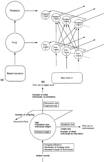
Fig. 1(a) shows the basal model structure of this study. Trophic energy or resources flow from lower levels to upper levels and out to environ-ment. In this study, the upper two levels are mainly analyzed as predator-prey system though there are three trophic levels formally. The lowest level is settled as constant volume in each calcula-tion just to rule the prey carrying capacity.
Fig. 1(b) shows the detailed view of the model. Each level has over-lapped generations with age structure and cohorts are functional units for dynamics. They compete within their level to sat-isfy their demand. They bear new offspring at reproductive periods and offspring from all co-horts makes one new cohort.
described in more detail in a later paragraph. The other two are population size and individual weight. These two enable us to distinguish mass and number of population. The age is added one every step and the population size and the individ-ual weight are recalculated according to gain or loss at every step.
2.1. Parameters
There are three trophic flows into or out of a trophic level. The first is intake flow from the adjacent lower level. The second is outward flow to the adjacent upper level. The third is outward flow to outside of the trophic chain or web, which is composed of intake loss, metabolism loss and death not caused by predator but by disease, accidental injury or starvation. And when cohorts are treated as functional units, one more flow between the units within each level is needed, presentation to newborns at reproductive period. Fig. 1(c) shows all fixed parameters (boxed) and calculating variables (bold) in this study.
For the first, minimum weight is defined for each age. It should be used as reference for birth, growth and death by starvation. Regarding the other parameters, they are associated with each trophic flow. For the first flow, cohorts act as consumer. In this model, three parameters are settled for action of consumer — that is maxi-mum of foraging trials, maximaxi-mum resource de-mand and foraging efficiency which means competitive coefficient which determines order of priority in foraging action among the same level individuals. For the second flow, the level acts as supplier. Two parameters are set for property of supplier, encounter rate to predator and captured rate when encountered. For the third flow, there are two different aspects. One is quantitative as-pect such as metabolism loss and intake loss. The other is numerical aspect that means individual death. As for intake loss, it was removed from intake volume by multiplying a fixed constant to the volume in all calculation. Metabolic loss was defined proportional value to three quarter power of weight in arbitrary unit, which is equivalent to unit of gain. For individual death, only starvation was considered and death by disease and
acciden-tal injury was excluded in order to drive the simulation by only trophic flow dynamics. Dead population by starvation is calculated through its weight referring to the minimum weight of its age. For the intra-level flow, which means propaga-tion by delivery and establishment of a new co-hort. No parameters are set for this flow because number of newborn is determined by individual weight and minimum weight of each cohort at reproductive period.
Actual value of parameters is determined as follows. For the first, minimum weight is defined for each age, according to growth curves of 3 and 7kg weight mammals for prey and predator, re-spectively. Then metabolism loss is defined pro-portional value to three quarter power of minimum weight in arbitrary unit, which is equiv-alent to unit of intake. This value means the minimum demand to live on. The maximum de-mand is settled as the value that has just enough surplus above metabolism loss in order to bear maximum number of offspring every reproductive period. These three fixed parameters are basically monotonous grow from birth to full grown up, and after grown up they are plateau. However, minimum weight just before reproductive period is raised by the surplus equivalent to requirement to bear one offspring per a couple per reproduc-tive period to assure that new generation would be born. The other parameters both as consumer, foraging efficiency and maximum of foraging tri-als and as supplier, encounter rate and captured rate are defined as fixed ones for each of the two species, predator and prey, respectively. They are determined arbitrarily, as populations that are at early reproductive age are advantageous in com-petition within the level.
2.2. Foraging trials
Predator’s foraging action is simulated as fol-lows. (1) One cohort of predator is chosen stochastically according to product of foraging efficiency and population size. (2) One cohort of prey is chosen stochastically according to product of encounter rate and population size. (3) Whether or not the predation between the preda-tor and the prey is successful is determined stochastically according to captured rate of the prey. (4) Three steps described above are repeated until maximal demand is fulfilled or foraging trial reaches the maximum during a unit time for every cohort of predator.
Though many predators with different foraging efficiencies will compete with one another and make trials to get a prey simultaneously in actual ecosystem, it is difficult to simulate as it is. There-fore, as an alternative method, a cohort of con-sumer is selected one by one sequentially according to competitive ability of each cohort. The product of foraging efficiency and population size of a predator cohort means relative size of the cohort that would be observed by internal observ-ers within the dynamics. When mass of prey that a cohort gets reaches per capita maximum de-mand, the population size of the cohort is sub-tracted one on calculating the product of foraging efficiency and population size. The probability that a certain cohort (Pi) is selected is:
Pi=FEi*PSci/S(FEi*PSci)
where FEi is foraging efficiency and PSci is popu-lation size of a cohort of consumer.
At the step 2, the product of encounter rate and population size of a prey cohort means relative size of the cohort that would be observed by internal observers within the dynamics. When to-tal prey population is small, predator may fail to find any of prey. When total prey population is large enough, predator can encounter one of prey without fail at every foraging trial. The probabil-ity that a certain prey cohort (Pj) is selected is:
Pj=ERj*PSsj/threshold (when threshold
\S(ERj*PSsj))
Pj=ERj*PSsj/S(ERj*PSsj) (when threshold
BS(ERj*PSsj))
where ERj is encounter rate and PSsj is popula-tion size of a cohort of supplier, threshold is relative size of the total supplier when it reaches saturation for consumer search.
If predation is successful, the selected cohort of consumer gets food by the individual weight of the chosen supplier and the number of foraging trials of the consumer population is added one, and the population size of the chosen supplier cohort is subtracted one. When predation is not successful, only addition to the number of forag-ing trials of consumer is performed. Every proba-bility used in these steps is calculated every time. On predation trial by prey, basically the same procedure as predation by predator is done. How-ever, as basal resource has only its volume, the probability on the second step (Search supplier) is defined as below.
P=1 (when thresholdBresource volume)
P=resource volume/threshold (when threshold
\resource volume)
And when a cohort of prey finds a basal re-source, it can be taken without fail. The resource volume decreases every successful predatory by prey.
2.3. Growth and propagation
Growth and propagation is calculated accord-ing to gain and loss of each cohort. Numbers of birth and death by starvation are determined by comparing individual weight of each cohort with minimum weight of its age.
num-ber and then monotonically decreases by preda-tion and starvapreda-tion.
At reproductive period, if one’s weight has surplus over the minimum weight of its age, it will bear its offspring according to the surplus. Off-spring from all reproductive age populations are gathered and make a new cohort. The weight corresponding to babies and secundina is sub-tracted from individual weight of the parental populations according to the number of offspring. Reproductive period comes every four step times for prey, and every 12 step times for predator. Maximum of brood size is six for prey and seven for predator. Prey can be reproductive from age eight to 48 every four period. Predator can be reproductive from age 12 to 96 every 12 period.
3. Dynamics
On fixed basal resource volume that range from 1×10⁴ to 4×10⁵, the dynamics of prey
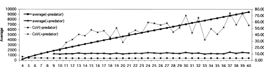
popula-tion only and both prey and predator populapopula-tions are calculated. The dynamics of prey population starts from one cohort of 10 young prey individu-als as the initial condition and has calculated for 400 steps on each basal resource volume. The last 300 steps are used for analysis. The dynamics of predator-prey system starts with the total popula-tion of prey at the last step of the prey only dynamics and one cohort of 10 young predator individuals as initial conditions. The dynamics has calculated for 1350 steps on each basal resource volume. And the last 1200 steps are used for analysis. Fig. 2 shows average and CoV
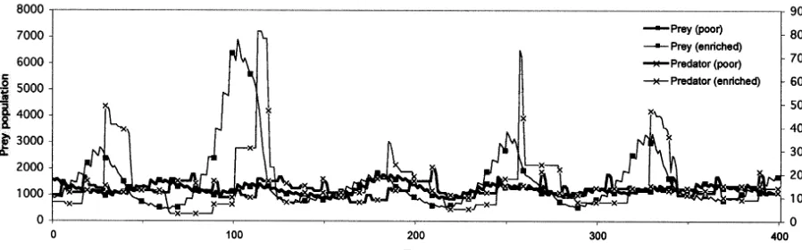
(coeffi-cient of variance) value of total prey population size on the population dynamics with or without predator as a function of basal resource. And Fig. 3 shows the population dynamics at 1×10⁵
(rela-tively poor condition) and 3×10⁵
(relatively en-riched condition) of basal resource.
Prey population can live on over 4×10⁴
of basal resource and 9×10⁴
or more of basal re-source is needed to support predator population on prey population. The average of total popula-tion size of prey without predator increases but the CoV value of that is flat as the volume of basal resource increases. On the contrary, on dy-namics with predator, increase of the average of population size of prey is limited but the CoV value of that increases as the volume of basal resource increases. It means that the paradox of enrichment is clearly observed on this model dy-namics. On the other hand, however, the increase of the CoV value accompanied with enrichment of basal resource is not monotonous. Though the amplitude of population size oscillation under the enriched condition is larger than that under the poor condition, the height of peaks on the en-riched condition varies at every surge. Under the enriched condition, the population size of prey may sometimes blows up to near the size without predator on the certain basal volume and can sometimes stay around the equilibrium of flows in and out for rather long duration. It means that the basal resource volume determines the highest peaks of prey population size, and the maximum amplitude of oscillation and the CoV value grow as the volume of basal resource grows. On the other hand, the equilibrium of flows is determined
Fig. 3. Population dynamics on poor and enriched conditions produced by individual base model.
by only interaction between prey and predator populations when basal resource volume is higher than the volume that preys need for the equi-librium. When the duration that the population sizes are kept around the equilibrium is so long that the CoV value is kept relatively low.
4. Domination on inter-level flow
To see which consumer or supplier is the domi-nant causation to control inter-level flow, it is calculated how much inter-level flow volume in-creases or dein-creases when prey or predator popu-lation size changes. For the first, the inter-level flow volume is calculated by total prey weight that is killed by predatory for serial 100 step. Then the inter-level flow volume is calculated at every 100 step as prey or predator population size varies by 10% each, from 60 (−40%) to 140% (+40%), independently. And ratio of the inter-level flow volume at 140%/that at 60% at every 100 step is also calculated. These calculations are made under the poor condition (basal resource volume 1×10⁵
) and the enriched condition (basal resource volume 3×10⁵
), respectively.
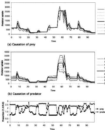
Fig. 4(a) and (b) show the range of inter-level flow volume for every 100 step under the poor condition by altering either of the prey or the predator population size, respectively, and Fig. 4(c) shows the ratio of flow volume at 140%/that at 60% for each 100 step. When the range is wide and the ratio is high, it means the altered
popula-tion is dominant at the step on determinapopula-tion of the flow volume. And on the contrary, if the altered population is less dominant or indepen-dent upon determination of the flow volume, the range should be narrow and the ratio low. The original flow volume at 100% shows major peaks every 12 months and some minor peaks every four months. The major peaks every 12 months correspond to predator reproductive periods and the minor peaks do to prey reproductive cycle though minor peaks would sometimes be unrecog-nizable and flat. The range from 60% to 140% by altering prey population is narrow, especially the upper range from 100% to 140%, except the dura-tion of major peaks. On the other hand, the range by altering predator population is wide and the upper range width over 100% and the lower range width below 100% are substantially the same though the upper range become small during the major peaks. The ratio of flow volume at 140%/
that at 60% in prey is low around 1.0 but raised during the predator reproductive periods. And that in predator is higher than 2.3 and slightly brought down at its reproductive periods. These results indicate that, under the poor condition, the consumer causation is mainly dominant on the determination of inter-level trophic flow and that the supplier causation is effective only just after predator’s reproductive period that the consumer population is crowded by new born offspring.
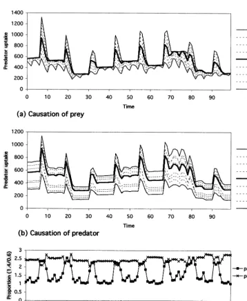
predator population size, respectively, and Fig. 5(c) shows the ratio of flow volume at 140%/that at 60% for each 100 step. Even under the enriched condition, the consumer causation is mainly dom-inant on the determination of inter-level trophic
flow all through population size oscillation. How-ever, during the shrinking phase after the peak of population size, the contribution of supplier cau-sation is relatively high and during growing phase, the contribution of prey less effective.
Fig. 5. Limitation on predator intake volume on the enriched condition. (a) Causation of prey,(b) causation of predator and (c) comparison between causation of prey and predator.
5. Discussion
5.1. Prey dependent, ratio dependent or predator dependent
There has been presented two types of predator-prey models, predator-prey-dependent model and
ratio-dependent model. The former describes that functional response of predator as function of prey density and the latter does as function of prey/
Prey-dependent models are essentially based on Lotka – Volterra equations that assume homoge-neous individuals. They have been employed ex-tensively as conventional models of predator-prey system. Since the functional response describes the behavior of searching predators, the function is prey-dependent. Predator zero-growth isocline of such models is vertical to prey axis and the paradox of enrichment arises from the isocline.
Ratio-dependent models have several theoreti-cal aspects. Leslie (1948) and Berryman (1992) adopted a logistic predator equation that included predator-prey ratio. Arditi and Ginzburg (1989) arrived at ratio-dependent predation through modification of the functional response, and Gutierrez (1992) made a ratio-dependent model by combining the physiological process of energy allocation with random search for prey. Ratio-de-pendent models are built by considering different time scale between searching behavior and popu-lation growth and interference among predators, and their right slanting predator isocline can avoid the paradox of enrichment.
In this study, I made the individual base model, which has prey-dependent linear functional re-sponse and includes interference among predators and delay of population growth from resource intake by not functional response but calculation procedure. The structure of total predation in a unit of time is similar to one of ratio-dependent models, metabolic pool model (Gutierrez, 1992). However, it is only when both predator and prey populations are composed of a single cohort and abundance of prey is not enough for predator’s maximum consumption that the biomass of prey killed by predation is linear to the ratio of prey/
predator. As for the ratio in this study, the nu-merator is the expected value of killed prey biomass per one foraging trial and the denomina-tor is total of maximum of foraging trials of predator. According to prey abundance, demand of predator is measured in two ways. It is de-scribed by its maximum consumption with enough prey or evaluated by maximum number of foraging trials on resource shortage. Since the threshold between the two is different among predator cohorts, the killed prey biomass is not proportional to the ratio when several predator
cohorts exist. Regard for prey, change rate of expected value coupled by predation is different among prey cohorts according to their individual weight and ratio-dependency is skewed when there are several prey cohorts.
Besides these reasons, as cohorts of less com-peting ability reduce their population size rapidly, cohorts of more competing ability can get enough prey at most of steps. Therefore, the prey biomass taken by predator is determined by predator population.
5.2. Mass and number
Trophic flow dynamics is essentially mass dy-namics and population dydy-namics is dydy-namics of number. Therefore, trophic population dynamics includes complicated relation between mass and number. For example, the inter-level flow between prey and predator means decrease of number for prey and increase of mass for predator. It is an important problem how to interpret flow mass into change of population size in number and how to estimate effect of number of population on mass of flows.
Predator-prey trophic models previously de-scribed as mathematical equations have solved it simply by treating all values as mass. The model of this study, each value of stock and flow keeps its character as number or mass. However, in total population size, there is not definitive differ-ence between mathematical models and the model of this study since total biomass is nearly parallel to population size because the range of individual weight is not wide through major part of popula-tion. As for predatory, foraging behavior of this study is just prey-dependent and assumptions on ratio-dependent theories are also included.
individual weight cannot be kept over minimum weight, the decline of mass is interpreted into the decline of number as death by starvation. If predator population has no structure and each individual is identical, as is the case on mathemat-ical models, it is possible that all individuals should die at once by just a mouthful shortage. It is of major importance that the predator popula-tion consists of sub-populapopula-tions that have differ-ent status in competitive ability. That means that some should die rapidly and that some should manage to survive rather long on small prey population.
In the introduction, three explanations are stated about inconsistency between theory and observation on the paradox of enrichment. This model proposes the fourth explanation that predator has several classes that has different vulnerability to starvation. Since the model of this study has one prey species, here would be no discussion about the first explanation that the prey consists of two species of edible and inedible. Efficacy of the second explanation, prey has in-vulnerable class, is confirmed again. In this study, prey population has age structure and cohorts at early reproductive age are less vulnerable. This feature forms temporal refuge. When the vulnera-bility is fixed for all ages, the range of the basal resource volume that allow predator population to last is very narrow because of typical paradox of enrichment effect (data not shown). As well as prey, the predator cohorts of young adult are advantageous in intra-species competition. This temporal refuge for predator is essential to the sustainability and when the parameters for forag-ing activity are constant for all ages, predator can persist for only short duration and then extinct (data not shown). This means the third explana-tion, the predator population density has a nega-tive effect on its own per capita population growth rate, is insufficient by itself. It is needed to stabilize predator-prey system that the negative effect of interference among predator should ap-pear in heterogeneous predator population. That is the fourth explanation proposed here.
At the equilibrium condition, mathematical models indicate per-capita growth rate is zero in biomass density, i.e. mass value. But individual
base model needs balance in number, too. It is necessary to accomplish the equilibrium that some predator individuals can reproduce their offspring with getting enough resource and some are going to die by resource shortage at the same time.
5.3. Per-capita approach and indi6idual base
approach
Because population dynamics arises from inter-actions between individual organisms, Berryman (1981) and Getz (1984) have argued that the equations should be derived as per-capita rates of change and the models are ratio-dependent type. The individual base model is similar to the per-capita model at the point of focusing on individ-ual attitude. Concepts and assumptions used in this study are not new except for the individual base, successive calculation structure. In spite of the same assumptions, the results are definitely different. The inter-level flow between predator and prey depends on neither prey density nor prey-predator ratio but the number of predator. And it is shown that heterogeneity in predator population is essentially important in persistency and stability of predator/prey system.
over-equilibrium prey without recursive and long lasting numerical increase.
Mathematical equation model is built from the viewpoint of outside observer. On the other hand, individual base, successive calculation model is constructed on the viewpoint of inside observer. Organisms are essentially inside observers and their behavior is dependent on not only their environment but also their own state and deci-sions. There are two partings of ways in calcula-tion procedure of the individual base model. One describes limitation of consumption and means consumer can cease foraging by its decision. The other describes the turning point on effect of resource shortage from loss of weight to death. Both reflect peculiar response of organisms that they may show different reactions under the same environment. These reaction changes make dis-continuity and the point of change is not stable. The individual base model is able to reflect status of individuals and represent the discontinuity pre-cisely, whereas per-capita models can hardly since they integrate various responses into one ‘per-cap-ita rate’. This integration is the parting way be-tween the individual approach and per-capita approach.
6. Conclusion
The model in this study is constructed based on individual behavior as consumer. Foraging trials will repeat until killed prey biomass reaches maxi-mum consumption of predator or the number of trials reaches maximum in a unit of time. These two limitations and the discontinuity between them are judged by consumer side. Only con-sumer can decide to make a foraging trial. In addition to this, the other discontinuity on re-source shortage is mainly associated with predator since prey should be eaten by predator so that prey would merely meet resource shortage.
Many of works about the paradox of enrich-ment have focused on the prey refuge i.e. spatial or temporal heterogeneity in prey population. But in this study, it is indicated that consumer cau-sation is dominant on inter-level flow volume and heterogeneity amongst predator is important on
persistency and stability of predator-prey systems. Therefore, the diversity of predator is no less important than that of prey in stabilization of the predator/prey dynamics. The focus of analysis for predator/prey system should also be put on predator.
References
Abrams, P.A., 1994. The fallacies of ‘ratio-dependent’ preda-tion. Ecology 75, 1842 – 1850.
Abrams, P.A., Walters, C.J., 1996. Invulnerable prey and the paradox of enrichment. Ecology 77, 1125 – 1133.
Arditi, R., Ginzburg, L.R., 1989. Coupling in predator – prey dynamics: ratio-dependence. J. Theor. Biol. 139, 311 – 326. Berryman, A.A., 1981. Population systems. Plenum, New
York.
Berryman, A.A., 1992. The origin and evolution of predator-prey theory. Ecology 73, 1530 – 1535.
Berryman, A.A., Gutierrez, A.P., Arditi, R., 1995. Credible, parsimonious and useful predator-prey models — a reply to Abrams, Gleeson and Sarnelle. Ecology 76, 1980 – 1985. Gause, G.F., 1934. The Struggle for Existence. Williams and
Wilkins, Baltimore.
Getz, W.M., 1984. Population dynamics: a per-capita resource approach. J. Theor. Biol. 108, 623 – 643.
Gilpin, M.E., 1972. Enriched predator-prey systems: theoreti-cal stability. Science (USA) 177, 902 – 904.
Gilpin, M.E., 1975. Group Selection in Predator – Prey Com-munities. Princeton University Press, Princeton.
Gutierrez, A.P., 1992. Physiological basis of ratio-dependent predator-prey theory: the metabolic pool model as a paradigm. Ecology 73, 1552 – 1563.
Huffaker, C.B., 1958. Experimental studies on predation: dis-persion factors and predator – prey oscillations. Hilgardia 17, 343 – 383.
Kretzschmar, M., Nisbet, R.M., McCauley, E., 1993. A preda-tor-prey model for zooplankton grazing on competing algal populations. Theor. Population Biol. 44, 32 – 66. Leibold, M., 1989. Resource edibility and the effects of
preda-tors and productivity on outcome of trophic interactions. Am. Naturalist 134, 922 – 949.
Lotka, A.J., 1925. Elements of Physical Biology. Williams and Wilkins, Baltimore.
Matsuno, K., 1995. Consumer power as the major evolution-ary force. J. Theor. Biol. 173, 137 – 145.
Matsuno, K., Ono, N., 1996. How many trophic levels are there? J. Theor. Biol. 180, 105 – 109.
May, R.M., 1972. Limit cycles in predator – prey communities. Science (USA) 177, 900 – 902.
Murdoch, W.W., 1994. Population regulation in theory and practice. Ecology 75, 271 – 287.
Hydro-biol. 73, 310 – 333.
Pimm, S.L., 1982. Food Webs. Chapman and Hall, London. Pimm, S.L., 1991. The Balance of Nature? University of
Chicago Press, Chicago.
Royama, T., 1992. Analytical Population Dynamics. Chapman and Hall, London.
Rosenzweig, M.L., 1971. The paradox of enrichment: destabi-lization of exploitation ecosystems in ecological time. Sci-ence (USA) 171, 385 – 387.
Sarnelle, O., 1994. Inferring process from pattern: trophic level
abundances and imbedded interactions. Ecology 75, 1835 – 1841.
Scheffer, M., de Boer, R.J., 1995. Implications of spatial heterogeneity for the paradox of enrichment. Ecology 76, 2270 – 2277.
Volterra, V., 1926. Variazioni e fluttuazioni del numero d’indi-vidui in specie animali conviventi. Mem. Acad. Lincei 2, 31 – 113.
Yodzis, P., Innis, S., 1992. Body size and consumer-resource dynamics. Am. Naturalist 139, 1151 – 1175.
.