Vol. 41 (2000) 85–99
The competition of user networks: ergodicity, lock-ins,
and metastability
Bernd Woeckener
∗Department of Economics, University of Tübingen, Mohstraße 36, D-72074 Tübingen, Germany Received 2 April 1998; accepted 27 May 1999
Abstract
This paper models the competition of user networks as a continuous-time Markov process. It presents a dynamic version of the Discrete Choice Analysis with state-dependent choice proba-bilities. Among other things, we show that the network competition can be characterized by the coexistence of lock-in regimes and a ‘metastable’ state — i.e. a state which is a probability max-imum for an arbitrary long but finite length of time. Then, unlike in the case of ergodicity or of simple lock-in scenarios, the networks can coexist for a considerable time span, although the market is a natural monopoly. ©2000 Elsevier Science B.V. All rights reserved.
JEL classification:D11; L10
Keywords:Ergodicity; Lock-in; Metastability; Network effects; Networks
1. Introduction
Often the utility from the use of a good depends positively on the total number of users of this good. In this case, the totality of users of this good constitute a user network. Obvious examples are communication systems such as fax and e-mail systems. Here a growth in the number of users directly induces positive network effects, because then each user can contact and be contacted by more users. Moreover, most information processing systems and a lot of consumer electronics systems are characterized by network effects as well. Clear examples are hardware–software systems such as computer systems or home video systems. Here the network effects are market-mediated: an increasing number of users leads
∗Tel.:+49-7071-2973-247; fax:+49-7071-2950-71.
E-mail address:[email protected] (B. Woeckener).
to a rising variety of software, and this in turn results in a higher utility of each user. The following analysis of the competition of two incompatible user networks,AandB, focuses on those cases where the choice of a network is not binding. A user’s decisions are modeled as a sequence of discrete choices which are, due to the network effects, state-dependent. Furthermore, in line with the Discrete Choice Approach, his willingness to pay is subject to exogeneous information and/or technology shocks, so that his choices are guided by state-dependent choice rates. In order to take into account that the user can review and revise his last choice whenever he wants, we treat time as a continuous variable, i.e. we follow a Master Equation Approach.
Our analysis shows that three qualitatively different outcomes are possible. Firstly, the probability distribution of the network sizes can converge to a unique continuous stationary distribution, i.e. the stochastic processes can be ‘ergodic’. Otherwise either one of the two boundary states ‘all users are in networkA’ and ‘all users are in networkB’ is a unique probability mass ‘absorbing’ state or both these states are absorbing. Here two cases have to be distinguished. In the first case, the absorbing state(s) is (are) the only equilibrium point(s) of the corresponding deterministic model. Then there is a strong tendency towards the realization of a monopoly, i.e. the stochastic process is quickly ‘locked in’ to one of the networks. In the second case, the absorbing state(s) is (are) accompanied by a ‘metastable’ state which corresponds with a stable interior equilibrium of the corresponding deterministic model. Then this state can be a probability maximum for an arbitrary long time span, i.e. the competing networks can coexist for a considerable period of time, although the market is a natural monopoly. This can only happen if it is taken into account that network effects typically decrease with increasing network size, i.e. that the rise in each user’s willingness to pay for a network induced by an additional user is smaller the larger the network is.
Pioneering work in the modeling of consumer behavior as a stochastic process with state dependence is Smallwood and Conlisk (1979) and Arthur et al. (1987). There, however, discrete-time processes are analyzed.1 Furthermore, the nonlinear Polya processes popu-larized by Arthur are restricted to the modeling of irreversible choices. Our continuous-time approach with endogenous review rates follows the Master Equation Approach presented in Weidlich and Haag (1983).2 However, whereas usually the transition rates of the stochas-tic processes are specified by behavioral assumptions, we present a version of the Master Equation Approach in which they are microfounded along the lines of the Discrete Choice Approach (for the latter, see de Palma and Lefevre, 1983). The central aim of our paper is to introduce the concept of metastability into economic analysis. Following van Kampen (1992), p. 328, ‘metastability’ denotes the coexistence of absorbing boundary states with a stable interior equilibrium state of the corresponding deterministic model which is a local probability maximum of the stochastic process for an arbitrary long but finite time span. We see this concept as central for the understanding of the evolution of markets for network effect goods, because it can explain the often observed long-term coexistence of competing user networks against the background that almost every user network has to exceed a critical mass, i.e. that in most cases both lock-in regimes exist.
1See also the related work of Kirman (1993) and Orl`ean (1995).
In Section 2 the choice rates are derived and aggregated to a master equation. In Section 3 we analyze the cases of ergodicity and of lock-ins in the absence of metastable states under the assumption that the network effects are approximately constant. Finally, in Section 4, we allow for the fact that network effects are typically decreasing and discuss the concept of metastability.
2. The model
2.1. Basic assumptions
Our model of the competition of two user networks aims at analyzing those cases in which the network choice is not binding and where each user can review and revise his choice whenever he wants. We have in mind users who, for example, own both a console for video-game cartridges and a PC with a CD drive (i.e. both hardware components), and who have to decide on whether they next buy a video game or a PC game (i.e. which kind of software to buy next). The current network membership of a user is determined by his last software choice, and the last software choices of all users determine the current network sizes. For simplicity, the total ‘mass’ of users is normalized to one, so that the total size of a network is identical with its market share. Furthermore, we suppose that the total number of users is very high and that they cannot coordinate their choices.3 As for the basic product characteristics, the two networks are assumed to be horizontally differentiated à la Hotelling with network Aat the left-end point and networkB at the right-end point of the unit line; i.e. networkAhas addressi=0 and networkBhas address i=1.
A user’s willingnesses to pay for being a member of networkAand for being a member of networkBconsist of two parts, the ‘basic’ willingness to pay which depends on product characteristics and that part which goes back to direct and/or market-mediated network effects and which is subsequently called ‘network effect function’:
• With regard to the basic willingness to pay, we assume that it is, at each point of time, uniformly distributed along the Hotelling line, where the address 0 ≤ i ≤ 1 of a user refers to his relative preference for a network as far as product characteristics are con-sidered (but not network sizes). The horizontal alienation effects (‘transportation costs’) are linear with regard to the distance betweenA(ati=0) orB(ati=1) and the user’s address. Hence, the alienation terms amount to−hi with respect to networkAand to −h(1−i)with respect to networkB, where the parameterhcan be seen as a measure of the extent of horizontal product differentiation. Taking into account address-independent partskAandkB, we obtain for networkA,kA−hi, and for network B,kB−h(1−i). We suppose that networkAcan have a systematic quality advantage, so thatkA ≥ kB holds.
• With regard to the network effect function, i.e. that part of the willingness to pay which goes back to the network effects, we assume that users do not differ in their valuation
3For a model with two groups of users with conflicting preferences where the users of each group can perfectly
of the network effects and that the network effects are constant (c = 1) or decreasing (c <1; the former is considered as an approximation for only modestly decreasing net-work effects). Hence, withx and 1−x as the size (market share) of networkAand networkB, respectively, the network effect functions readnxcforAandn(1−x)c for B, where the parameternis a measure of the ‘network effect strength’. This parameter shows how strong the positive relationship between the demand for (size of) a network and the willingness to pay for being a member of this network is. Its value depends, among other things, on the size of the fixed costs of software production. The lower the fixed costs of introducing a new software variant are, the more new variants are induced by a certain increase in demand.
Considering current user costsgAandgB, we presume that the (eventual) systematic quality advantage of networkAis not overcompensated by higher costs, so thatkA−gA≥kB−gB holds. In the following, the differencekA−gAis denoted asaAand the differencekB−gB asaB. Hence, the difference between a user’s total willingness to pay for being a member of networkAorBand its current user costs — i.e. his current surplus from being a member of the respective network — can be formulated as
siA=aA+nxc−h i (1)
and
siB=aB+n(1−x)c−h(1−i), (2)
respectively. Here, the differenceaA−aB≥0 is the ‘systematic basic advantage’ of network Aand is subsequently denoted asb. It is the systematic part ofA’s ‘basic advantage’bi = b+h(1−2i)(which can be negative).
choosing networkAand for choosing networkB are the same for all users (at a point in time).4
2.2. The individual decisions: choice probabilities
A user with current (new) addressichoosesAwheneversiA > siB holds. Using Eqs. (1) and (2), this condition can be formulated as−b−h(1−2i)≤n[xc−(1−x)c]. Thus, networkAis chosen wheneverB’s basic advantage−bi = −b−h(1−2i)is smaller than (or equal to)A’s ‘network size advantage’n[xc−(1−x)c]. Asiis uniformly distributed between zero and one,B’s basic advantage is uniformly distributed between−b−hand −b+h. Hence, its cumulative distribution is
K(−bi)=
By substitutingA’s network size advantage forB’s basic advantage, we obtain the choice probabilities of networkAas
The choice probabilities of networkBareβ(x)=1−α(x). These state-dependent choice probabilities are the probabilities that networkAorBis chosen given that a user, due to an exogeneous shock, reviews his last choice. For the special case of constant network effects (c=1), we obtain
2.3. The evolution of networks: master equations
In order to derive the equations of motion for the probability distribution ofA’s network sizex, let us suppose (for a moment) that time is a discrete variable. Let us further assume that the process is a one-step process, i.e. that in fixed time intervalsτ(only) one of the users reviews his choice (on the occasion of a software purchase). Moreover, let the probability of doing so be the same for each user, and letǫbe the inverse of the number of users. Then if at a point in timetthe statexis realized, the probability that at timet+τ the statex+ǫ
4This is the usual assumption in Discrete Choice Theory. However, there is a decisive difference between our
is realized amounts toA(x)=(1−x)α(x): a member of networkB reviews his choice (appears at the market) and chooses networkA. Analogously, the transition probability for transitions from statexto statex−ǫreadsB=xβ(x). If at timetone of the two neighboring statesx−ǫandx+ǫis realized, the transition probabilities for transitions to statex are
A(x−ǫ)=[1−(x−ǫ)]α(x−ǫ)andB(x+ǫ)=(x+ǫ)β(x+ǫ), respectively. Hence, the Chapman–Kolmogorov forward equation for this discrete-time Markov process is
P (x;t+τ )−P (x;t )=A(x−ǫ)P (x−ǫ;t )+B(x+ǫ)P (x+ǫ;t ) −[A(x)+B(x)]P (x;t ).
So far the time spanτ which elapses until a review takes place is constant and exoge-neously given. As we want to endogenize it, we pass over to continuous-time processes. In general this requires an expansion of the discrete-time transition probabilities in a Taylor series around a point in time and the subsequent calculation of its limit forτ →0 in order to obtain the continuous-time transition rates (hazard rates). In the case of our one-step process with (state-)discrete choices, however, every realization of the process after any small time intervalτ— no matter how small — retains the same value ofxwith a certain probability or attains a value which differs byǫ >0 with the complementary probability. Hence, the short-term behavior of a realization of the process is characterized by phases of constantx which are interrupted by jumps of sizeǫ >0. In the case of such a short-term behavior, the choice and transition rates differ from the choice and transition probabilities only with regard to their general level, i.e. they are of the same functional form (see Honerkamp, 1994, p. 171f). Thus, with 0< θ <1, the master equation of the corresponding continuous-time Markov process can be written as
˙
P (x;t )=θ{(1−x+ǫ)α(x−ǫ)P (x−ǫ;t )(x+ǫ)β(x+ǫ)P (x+ǫ;t )
−[(1−x) α(x)+xβ(x)]P (x;t )} (5)
for all 0≤ x ≤ 1 and withP (x;˙ t ) =∂P (x;t )/∂t. This master equation can be seen as a probability flux balance, where the first line yields the probability influx into a statex, and the second line yields the probability outflux from this state. In the following, in order to avoid notational clutter, we rescale time with 1/θ. Formally, this means dividing the right-hand side of Eq. (5) (but not the left-hand side) byθ.5
In the absence of network effects, i.e. with constant choice rates αandβ, the master equation would be linear inx and a closed differential equation system for the motion of all moments of the probability distribution could be derived from it (see van Kampen, 1992, p. 149ff). Forn > 0, no such explicit dynamic solution is feasible. However, an approximate solution can be obtained insofar asx is a quasi-continuous variable and as long as the transition rates are continuously differentiable. Then the master equation can be approximated by a state-continuous Fokker–Planck equation, from which we can derive a differential equation system for the moments. While the first condition is, due to our assumption of a high total number of users, always fulfilled, the second condition requires
5This normalization allows us to use the same symbols (α,β,n,h, etc.) for the probabilities/rates and parameters
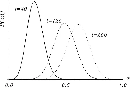
Fig. 1. Transient probability distributions of an ergodic process forx0=0 (c=1,h=1,n=0.5,b=0.2).
that the choice rates do not take on the values zero and one. If the latter is not fulfilled, the nonlinear process can be analyzed by means of its corresponding deterministic model (the ‘macroequation’). In the next section both the approximate solution via the Fokker–Planck equation and the analysis via the corresponding deterministic model is carried out for the case of (approximately) constant network effects.
3. Network competition with constant network effects: ergodicity versus lock-ins
3.1. Ergodicity
In the case of constant network effects, the choice rate of networkB remains positive withx =1 forn < h−b(and the choice rate of networkAremains positive withx =0 forn < h+b; see Eq. (4)). Then the transition rates are continuously differentiable and the master equation can be approximated by a state-continuous Fokker–Planck equation. The conditionn < h−bis met if bothn < handb < h−nholds, i.e. if the network effects are ‘relatively weak’ (compared to the extent of the horizontal differentiation or exogeneous shocks) andA’s systematic basic advantage is ‘relatively low’ (compared to the difference between the extent of the horizontal differentiation or exogeneous shocks and the network effect strength). Then sooner or later all states have a positive probability of being realized, so that every process is sooner or later characterized by a continuous probability distribution which covers all states.
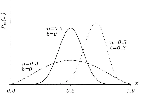
Fig. 2. Stationary probability distributions of three ergodic processes (c=1,h=1).
probability of a state is equivalent to its relative frequency realized in the course of time; this is the ‘ergodic property’ (see van Kampen, 1992, p. 93). Therefore, the moments of the stationary probability distribution are of the same value as the moments calculated from a realized trajectory (provided that it is long enough). Obviously, ergodicity of the stochastic process means coexistence of competing user networks.
In order to obtain some general results, we derive the state-continuous Fokker–Planck equation by expanding the master equation as a Taylor series up to the second-order term.6 This leads to
˙
P (x;t )= − ∂
∂x[D(x)P (x;t )]+ ǫ 2
∂2
∂x2[F (x)P (x;t )] (6)
with
D(x)=A(x)−B(x)=α(x)−x =0.5+b−n 2h +
n
h −1
x (7)
and
F (x)=A(x)+B(x)=(1−x)α(x)+xβ(x)=0.5+b−n 2h +
2n−b h x−
2n h x
2. (8)
The driftD(x)can be interpreted as the systematic part of the process, and the fluctuation termF (x)as the influence of the random shocks. By multiplication of the Fokker–Planck equation withxorx2and subsequent partial integration, we obtain the dynamic mean-value equation as
h ˙xi = hD(x)i, (9)
and the differential equation for the second moment results ash ˙x2i =2hxD(x)i +ǫhF (x)i.
6For the general procedure of the derivation of a Fokker–Planck equation and its moment equations, which are
Hence, the differential equation for the variance is
hh ˙x2ii =2hxD(x)i +ǫhF (x)i −2hxihD(x)i. (10)
From Eq. (9), it becomes clear that the drift of the stochastic process gives the best pos-sible approximation for the most probable trajectory of a realization. Withh ˙xi = 0, we obtain (the best approximation of) the most probable state after the stationary distribution has been reached:
hxi∗=0.5+ b
2(h−n). (11)
According to Eq. (10), the variance of the stationary distribution is
hhx2ii∗= ǫh
Hence, a higher systematic basic advantageb(withb < h−n) ofA, for example due to lower software prices, leads on average to a higher network size ofAas well as to a lower variance. The two stationary distributions forn=0.5 depicted in Fig. 2 provide an example. From Eq. (11), we can deduce that network effects work like a multiplier of a systematic basic advantage and that a higher network effect strength (withn < h) results on average in a larger size ofA(givenb >0). Moreover, as long asbis not too high, a highern means a higher variance, i.e. stronger network effects make the network competition more uncertain. Fig. 2 provides an example forb=0.
The driftD(x)serves not only as the approximate mean-value equation but also as the corresponding deterministic modelx˙ = α(x)−x of the process. Its equilibriax∗ result from Eq. (11) and, as long as the process is ergodic, the following correspondence holds (cf. van Kampen, 1992, p. 254ff): stable equilibria of the deterministic model correspond with (local) maxima of the stationary distribution of the stochastic process, and unstable equilibria of the deterministic model correspond with local minima of the stationary distribution of the stochastic process. If the process is not ergodic, but rather absorbing states exist, the whole probability mass is absorbed by these states fort → ∞. Here stable equilibria of the deterministic model correspond with states which are (local) probability maxima for a finite period of time.
3.2. Lock-ins
member ofAappears at the market and choosesAagain or whether a member ofBappears and switches toA. However, sooner or later all users are members of networkA, i.e.x =1 is an absorbing state.
Whereas in this first case the final market outcome is always anA-monopoly, the second case is characterized by the fact that it is a priori uncertain which network will prevail. Here the network effects are relatively strong (n > h), and the systematic basic advantage is relatively low (b < n−h). In this case, both lock-in regimes exist, and the interior boundary state for lock-ins to networkBisxℓ,B=0.5−(h+b)/(2n). The two statesxℓ,A andxℓ,Bare the critical masses of networkBandA, respectively, which must be exceeded in order to enter the market. As in reality most user networks possess a critical mass, we subsequently focus on processes with both lock-in regimes.
Using Eq. (7) and taking into account the lock-in regimes, we obtain the corresponding deterministic model of the second case as
˙ x=
−x if x≤0.5−(h+b)/(2n) 0.5+(b−n)/(2h)+(n/ h−1) x otherwise
1−x if x≥0.5+(h−b)/(2n).
(13)
Here this deterministic model cannot be interpreted as an approximation of the mean-value equation, but it reflects some qualitative features of the stochastic process. It has three equilibria: x = 0,x = 1 and an interior equilibrium x∗ which can be calculated from Eq. (11). The two boundary equilibria are stable (the eigenvalues are∂x/∂x˙ = −1) and correspond with the absorbing states of the stochastic process. In contrast, the interior equilibrium is unstable (∂x/∂x˙ = n/ h−1 > 0 due ton > h). This means that every realization of the process with an interior initial conditionxℓ,B < x0< xℓ,Amore or less quickly enters one of the lock-in regimes.
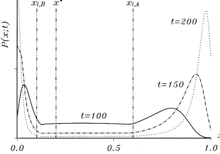
In Fig. 3, this is demonstrated for a stochastic process withh=1,n=2 andb =0.6. From Eq. (13), we can calculate that there are two large lock-in regimes withxℓ,B =0.1 andxℓ,A =0.6 and that the unstable interior equilibrium amounts tox∗=0.2. The three depicted transient distributions are calculated by means of the master equation (where we
Fig. 3. Transient probability distributions of a process with both lock-in regimes forx0 =0.24 (c=1,h=1,
Fig. 4. Stationary probabilities of a lock-in toAfor two processes with both lock-in regimes (c=1,h=1). now have to take into account that inside the lock-in regimes the probability mass can flow in only one direction). Starting the process withx0=0.24, initially the distributions have a unique maximum near this state. But due to the competition of the absorbing boundary states for probability mass, they soon become bimodal. In the first stage, there are two local interior maxima inside the lock-in regimes, but both the absorbing states become most probable relatively quickly. As the process progresses, they absorb all probability mass beforet =500 is reached.
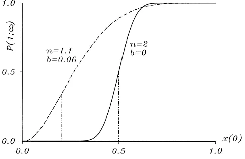
Fig. 4 depicts the influence of the initial condition, of the network effect strength and of the systematic basic advantage on the outcome of the network competition. There we have depicted the numerically calculated relationship between the stationary lock-in-to-A probability and the initial condition forn=2 andb=0 as well as forn=1.1 andb=0.06 (andh =1 in both cases). It turns out that these relationships are functions with turning points at the interior equilibria (which arex∗=0.5 andx∗=0.2, respectively). Of course, a higher systematic basic advantage of networkAdue to lower prices and/or higher quality shifts the whole function to the left. Moreover, the significance of the initial condition on the success probabilities of networkAis higher, the stronger the network effects are. In other words, stronger network effects make the process more deterministic.
4. Network competition with decreasing network effects: metastability
Usually, network effects become noticeably weaker with increasing network size. If this fact is taken into account, we can explain why competing user networks often coexist for a considerably long time, although one or both networks have a critical mass — i.e. although the market is a natural monopoly. The key for explaining this phenomenon is the concept of metastability: one or both lock-in regimes can coexist with an interior (local) probability maximum which can be arbitrarily long-lived.
i.e.(h+b)/n <1 results in the existence of a lock-in-to-Bregime.7In the case of ergodicity, it makes no qualitative difference whether the network effects are (approximately) constant or (noticeably) decreasing. In the presence of lock-in regimes, however, the existence of a metastable state changes the characteristics of a stochastic process considerably. As in the previous section, we focus on processes with both lock-in regimes.
If the network effects are constant, the eigenvalues of the corresponding deterministic models amount ton/ h−1 (as long asxℓ,B < x < xℓ,A), i.e. they arex-independent. In contrast, if the network effects are decreasing, not only the value of the eigenvalues is state-dependent, but also their sign can be state-dependent. Fromx˙=α(x)−xwithα(x) according to Eq. (4), we obtain
∂x˙ ∂x =
cn[xc−1+(1−x)c−1]
2h −1. (14)
This is a parabolic function with its minimum atx =0.5, where the minimum eigenvalue is∂x/∂x˙ =cn21−c/ h−1. Furthermore, lim
x→0∂x/∂x˙ =limx→1∂x/∂x˙ = +∞holds, i.e. for (very) low as well as for (very) highx-values, the eigenvalues are always positive. Hence, there are two parameter regimes:
• Forn/ h >0.51−c/c, the minimum eigenvalue is positive. Thenx˙is increasing over the entire rangexℓ,B< x < xℓ,A, so that there is either a unique unstable interior equilibrium or no interior equilibrium at all. Therefore, either one or both lock-in regimes exit, and the stochastic processes do not differ qualitatively from those discussed in Section 3.2. • Forn/ h <0.51−c/c, the minimum eigenvalue is negative. Herex˙is increasing for low
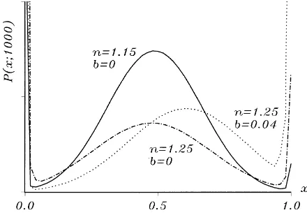
as well as for highx-values but decreasing in between. In this case, the deterministic model can have three interior equilibria: two unstable ones and between them a stable equilibrium. The latter corresponds with a metastable state of the stochastic process. Fig. 5 shows the corresponding deterministic models of three stochastic processes with c=0.5 andh =1 (calculated fromx˙ =α(x)−x withα(x)according to Eq. (4)). Two of them are symmetric (b=0), so thatx =0.5 is the stable equilibrium. Whilen=1.15 results in an unstable equilibrium atx =0.0275 as well as atx =0.9725 and has lock-in regimes withxℓ,B=0.015 andxℓ,A =0.985, a higher network effect strength (n=1.25) leads to larger lock-in regimes (see the blips of the functions) and to unstable equilibria which lie further inside. In the third example, networkAhas a systematic basic advantage of b=0.04, so that the stable equilibrium amounts tox =0.72. From the equilibria of these deterministic models, we can infer the qualitative properties of the stochastic processes and, thus, of a typical realization. Let us assume, for example, thatA’s network size is initially a little bit higher than its critical mass. Then, in the first stage, there is a considerably high probability that a realization will be locked in to networkB. If, however, networkA ‘survives’ this critical stage and succeeds in exceeding the state which corresponds to an unstable equilibrium of the deterministic model, it becomes increasingly probable that a realization fluctuates around the metastable state for a very long time.
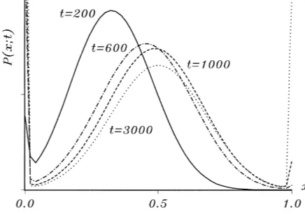
Fig. 6 provides an example forn = 1.15 and x0 = 0.2, i.e. with an initial state to the right of the left-hand unstable equilibrium. In this case, a long-term coexistence of
7In the special case ofc=0.5, the interior boundary states of the lock-in regimes can be calculated asx
ℓ,A=
0.5+[(h−b)/(2n)]p2−[(h−b)/n]2andx
ℓ,B=0.5−[(h+b)/(2n)]
p
Fig. 5. Corresponding deterministic models of three processes with a metastable state (c=0.5,h=1)
Fig. 6. Transient probability distributions of a process with a metastable state forx0 =0.2 (c= 0.5,h=1,
n=1.15,b=0).
Fig. 7. Transient probability distributions of three processes with a metastable state fort =1000 andx0=0.2
(c=0.5,h=1).
metastable state, where a monopoly is realized (with certainty) within a by far shorter time span.8
How strong the metastability is, i.e. how long competing user networks can coexist although the market is a natural monopoly, depends, among other things, on the general strength of the network effects. This is demonstrated in Fig. 7 via the comparison of the probability distributions fort = 1000 andx0 =0.2 of the processes withn =1.15 and withn=1.25. Obviously, stronger network effects mean a stronger tendency towards the driving out of one of the networks: the probabilities for being locked in (for being in the neighborhood of the metastable state) are higher (lower), the highernis. This can also be deduced from the corresponding deterministic models depicted in Fig. 5: a highernmeans larger lock-in regimes and a lower eigenvalue (in absolute terms) of the stable equilibrium. Finally, in order to illustrate the effect of the existence of a systematic basic advantage of networkA, Fig. 7 shows the probability distribution fort=1000 andx0=0.2 which results fromb =0.04. Here the peak of the interior distribution lies to the right ofx =0.5, and the probabilities for a lock-in toA(B) are comparatively high (low). Of special importance for realizations of this process are the relatively high escape probabilities for switches to x =1. These are due to the fact that the distance between the metastable state (x =0.72) and the state which corresponds to the right-hand unstable equilibrium of the deterministic model (x =0.81) is relatively small.
5. Conclusions
This paper applies a dynamic version of the Discrete Choice Model to the problem of competing user networks. In order to determine the evolution of the probability distribution
8Remember that for the parameter specification used in Fig. 3, a monopoly is realized (with certainty) before
of the network sizes, we have employed a continuous-time Master Equation Approach with state-dependent choice rates. We have shown how these nonlinear stochastic continuous-time processes can be analyzed by means of the moment equations of the Fokker–Planck equation and/or with the help of the corresponding deterministic model. It turns out that, depending on the strength of the network effects, the extent of the horizontal differentiation (the im-portance of the exogeneous shocks), the significance of a systematic basic advantage and on the curvature of the network effect function, four cases can be distinguished:
• If the systematic basic advantage is relatively high, a unique absorbing state exists, and, sooner or later, every realization of a stochastic process is locked in to the network with the systematic advantage.
• If both the systematic basic advantage and the network effect strength are relatively low, the stochastic processes are ergodic; i.e. every realization of a stochastic process results in a coexistence of networks.
• If the systematic basic advantage is relatively low and the network effects are considerably strong (given the curvature of the network effect function), both lock-in regimes but no metastable state exist. Hence, there is a strong tendency towards a quick driving out of one of both networks, and it is a priori an open question as to which network this will be. • If the systematic basic advantage is relatively low and the network effects are relatively strong but not considerably strong, the two lock-in regimes could coexist with a metastable state. Here if both networks have exceeded sufficiently their critical masses, a relatively long-lasting coexistence becomes probable, although the market is a natural monopoly. The latter can only happen when the fact that network effects are decreasing is taken into account. Unlike the second case, it can explain a long-lasting coexistence of user networks in the presence of critical masses.
References
Aoki, M., 1996. New Approaches to Macroeconomic Modeling. Cambridge University Press, Cambridge, UK. Arthur, W.B., Ermoliev, Y.M., Kaniovski, Y.M., 1987. Path-dependent processes and the emergence of
macro-structure. European Journal of Operational Research 30, 294–303.
de Palma, A., Lefevre, C., 1983. Individual decision-making in dynamic collective systems. Journal of Mathematical Sociology 9, 103–124.
Honerkamp, J., 1994. Stochastic Dynamical Systems, VCH, New York.
Kirman, A., 1993. Ants, rationality, and recruitment. Quarterly Journal of Economics 108, 137–156.
Orléan„ A., 1995. Bayesian interactions and collective dynamics of opinion: herd behavior and mimetic contagion. Journal of Economic Behavior and Organization 28, 257–274.
Smallwood, D.E., Conlisk, J., 1979. Product quality in markets where consumers are imperfectly informed. Quarterly Journal of Economics 93, 1–23.
van Kampen, N.G., 1992. Stochastic Processes in Physics and Chemistry. North-Holland, Amsterdam. Weidlich, W., Haag, G., 1983. Concepts and Models of a Quantitative Sociology. Springer, Berlin.
Witt, U., 1997. “Lock-in” vs. “critical masses” – industrial change under network externalities. International Journal of Industrial Organization 15, 753–773.
Woeckener, B., 1993. Innovation, externalities, and the state: a synergetic approach. Journal of Evolutionary Economics 3, 225–248.