STUDYING GLACIAL MELT PROCESSES USING SUB-CENTIMETER DEM
EXTRACTION AND DIGITAL CLOSE-RANGE PHOTOGRAMMETRY
E. Sanz-Ablanedo a, J. H. Chandler b, and T.D.L Irvine-Fynn c
a
Dept of Cartography, Geodesy and Photogrammetry, Universidad de León, Spain, –
[email protected] bCivil and Engineering Dept, Loughborough University, U.K. –
[email protected] cInstitute of Geography and Earth Sciences, Aberystwyth University, U.K.
– [email protected]KEY WORDS: Close-range photogrammetry, Glacier roughness, DEM extraction, Geomorphology
ABSTRACT:
Glaciers are sensitive to climatic variation and a particular developing area of investigation is in the field of "cryoconite”, referring to dustlike residues which form on the glacier surface. Cryoconite absorbs the Sun's shortwave energy, accelerates ice melt and because of the localised distribution of dust creates localised melting which is highly spatially variable. There is therefore a need to quantify the detailed topographic surface of ice and measure its variability through time. This paper describes the use of close range photogrammetry to reconstruct the glacier surface at the sub-centimetre or micro scale, an approach which may allow the relationship between cryoconite and ice surface properties to be explored over either space or time. The field campaign was conducted at Midtre Lovénbreen, Svalbard (78.88° North 12.08° East), during the summer of 2010 and executed using simple equipment and procedures. A simple and ageing Nikon 5400 5 MP camera was used to acquire all imagery, proving sufficiently robust for the challenging field environment. The camera was handheld approximately 1.6 m above the ice surface, providing an oblique perspective. Images were acquired at three different camera/object distances, each generating coverage occupying three different areas. All imagery was processed using the commercial photogrammetric package PhotoModeler Scanner, generating three-dimensional point clouds consisting of many thousands of XYZ coordinates, each colour-coded. It had been feared that lack of texture in the ice surface combined with differing specular reflections in each image would compromise the DEM generation process. Results were better than expected, although DEM quality proved to be variable depending on ice cleanliness and more significantly, the degree of obliquity of the image pairs. Despite these differences, digital close-range photogrammetry has proven to be a useful technique to reconstruct the glacier's surface to sub-centimeter precision. Moreover, the method is providing glacial scientists with new data to examine the relationship between cryoconite, ice surface roughness and melt processes.
1. INTRODUCTION
1.1 Cryoconite as a glacier melting agent
Glaciers are sensitive to climatic variation and both remote sensing and photogrammetry has been widely used to solve a range of problems relating to their dynamic geometry. For example, it has been possible to obtain valuable data concerning climate-forced change by studying glacial surfaces and both their modification and motion. One particular developing area of investigation is in the field of “cryoconite" which is a term used to refer to dust-like residues on glacier surfaces (e.g. Takeuchi & Li, 2010; Hodson et al., 2010; Bøggild et al., 2010). This dust not only comprises airborne mineral particles (e.g. local rock or distal desert sources) and pollutant particulates (e.g. black carbon) but includes a wealth of biological entities arriving from atmospheric sources as well as growing in situ. Cryoconite has high light absorbency and when distributed over the ice surface absorbs the sun's shortwave energy, converting it into heat and thus accelerating local ice melt (Takeuchi, 2002). Consequently, there is a subtle interplay between the planimetric proportion of cryoconite coverage and ice surface roughness which affects ice surface energy balance, and ultimately the glacier’s mass balance. For this reason there is a growing awareness of the glaciological significance of this supraglacial dust.
1.2 Glaciers roughness measurement
To study the influence of cryoconite glacier ice melt rates, it is necessary to know the detailed variation of the glacier's surface
over time, as impacts can be highly localised. Ice surface energy balance is sensitive to ice roughness at the metre to 10s of metres scale while at the sub-metre scale, roughness has implications on data retrieved by various satellite sensor arrays (Rees and Arnold, 2006). Traditionally, to quantify ice roughness, several control areas are chosen where the ice surface elevation is measured with a tape with respect to a horizontal reference plane (e.g. Brock et al., 2006). Due to the high resolution of detail required (centimeters), satellite or airborne sensors cannot be effectively used and indeed remain an expensive option. Similarly, the high number of control areas to be measured in a short time, the environmental conditions, the frequency of the measurements and the loss of returns from snow and water make terrestrial laser scanning impracticable. Digital close-range photogrammetry could provide both an economic and effective tool for determining variations in the surface of a glacier, particularly at close range using ground-based imagery. First, the necessary field equipment is reduced to a simple and comparatively cheap consumer grade digital camera. Secondly, the time required for data collection is reduced to that needed to acquire digital images. Subsequently, further data processing can be achieved in environmental conditions more comfortable than those that typically occur on a glacier.
This paper presents the results obtained from a field season conducted in Svalbard, which evaluates the performance of digital close-range photogrammetry for capturing glacial surface morphology.
2. GLACIER MEASUREMENT-PREVIOUS WORK
There is a long history of measuring glacial surfaces using remote sensing techniques. Baltsavias et al, (2001) provides a useful review including space-borne sensors, aerial photogrammetry and airborne laser and optical sensors. Space-borne sensors are suitable for iceberg tracking and glacier mapping or glacial mapping at small-scale but are unsuitable if a DEM is required. Airborne laser scanning and aerial photogrammetry have been successfully used for medium scale tasks. However, difficulties arise in airborne photogrammetry within areas exhibiting strong shadows, or where there are large expanses of white ice/snow, or smooth snow (Baltsavias et al., 2001; Fox and Gooch, 2001). Such areas cause gross errors in DEMs generated automatically using traditional area correlation techniques. Airborne laser sensors perform better on texture-less snow and ice areas, but blunders are likely in regions exhibiting poor reflectivity due to debris or rock (Baltsavias et al., 2001). Despite this, both airborne laser scanning and digital photogrammetry appear to be suitable for medium-scale cryospheric applications, retrieving roughness at the decimetre scale (Baltsavias et al. 2001; Nolin et al., 2002; Hopkinson and Demuth, 2006; Höfle et al., 2007; Rees and Arnold, 2006). The airborne perspective remains inappropriate for aerodynamic applications where a centimetre or millimetre scale is necessary.
Close range photogrammetry offers opportunities and work has been done in the past in relation to mapping small areas of glaciers at medium scale. For example, Kaufmann and Ladstädter (2008) monitored ablation occurring within a valley glacier by using a very wide range of imagery dated 1988-2007, including imagery acquired using consumer grade digital cameras.
Non-photogrammetric but measurement involving images has been conducted at very close range before. This has normally involved a thin black plate of known dimensions inserted into the snow or ice. This enables a continuous ice surface profile to be recovered from the high contrast digital representation, with horizontal resolutions between 1 and 3 mm reported (e.g. Rees, 1998; Arnold and Rees, 2004; Rees and Arnold, 2006). More recently, with the advent of higher-resolution digital cameras, horizontal resolutions for this method have improved further to 0.15 mm (e.g. Fassnacht et al., 2009; 2010) but this technique remains limited to singular 2D profiles. Interestingly, Fassnacht et al (2009) also refer to work conducted in soil science, where photogrammetry has played a leading role in deriving roughness measures which are of relevance to this project (Irvine-Fynn et al, In Prep.). Kirby (1991) recovered a set of profiles to represent the un-vegetated desert surface, consisting of either pebbles or sand. Rieke-Zapp and Nearing, (2005) used a six megapixel Kodak DCS1 digital camera to measure and monitor soil erosion within a 4 x 4m test facility. Taconet and Ciarletti, (2007) used a lower resolution DCS200 and generated their own area-based matching algorithm to measure agricultural soil surfaces within an area covering 0.8-1.1 m2. They identified several roughness indices, including: elevation standard deviation, slope angle and tortuosity index, and elevation auto covariance.
Ground based terrestrial laser scanning (TLS) has been trialled for snow and glacier surfaces (Kerr et al., 2009; Kaasalainen et al., 2011). From such data, profiles recording surface topography can be retrieved at centimetre-scale horizontal and millimetre-scale vertical resolution, over intermediate scan distances (< 200 m). However, as Hopkinson (2004) noted, the success of TLS on ice surfaces can be influenced by factors
including the angle of incidence, specific laser wavelength and the associated signal loss on the varied surface materials and textures in supraglacial environments, and the duration of scanning itself.
3. EXPERIMENTAL DESIGN
3.1 Capturing data
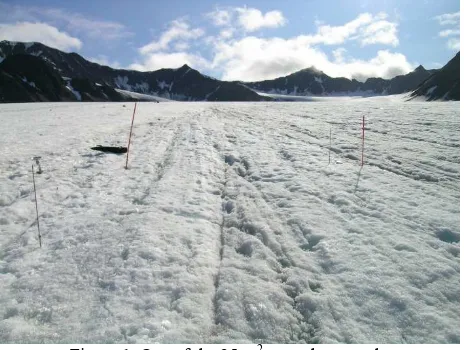
The study presented here was conducted on Midtre Lovénbreen (78° 52’N, 12° 05’E) during the summer of 2010. At site RC3, a location on Midtre Lovénbreen’s centre line, at ~ 200 masl, a 2.5m pole was drilled and secured such that the base of the pole froze into the ice (Figure 1). Because of the heightened heat conduction of metal, a polyethylene pole was used. The pole was marked to provide a fixed reference point for all surveys at the site. Two taut 5 m survey strings were tied from the anchor pole to temporary vertical poles secured with ice screws. This provided an approximately horizontal reference plane. The strings, marked at 0.5 m intervals, were oriented at approximately 90°, with one perpendicular to the ice surface slope and prevailing wind direction, and the second aligned in the down glacier direction (Figure 1).
Figure 1. One of the 25 m2 area photographs
Imagery was acquired obliquely from eye-level (~1.6m; see Figure 1 and Figure 2) and no support was used to raise the height of the camera further. Three pairs of convergent photographs were taken using a 5MP Nikon 5400 consumer grade digital camera. This camera has a sensor of 7.5x5.3mm and a minimum focal lenth of 6.2mm, so the vertical field aperture is approximately 46. The photos were captured from a distance allowing coverage of the entire area of interest by a single image and initial camera orientation was chosen so that the position of the reference pole occupied the upper left area of each image. Plot areas of 25 m2 (Figure 1), 4 m2 (Figure 2) and 1 m2 (Figure 3) were acquired and an approximate base-to-distance ratio of five was chosen, to create a suitable set of stereo-pairs necessary for DEM generation at the three scales. Images were acquired typically during early afternoon at one-week intervals over a period of six one-weeks.
3.2 Camera Calibration
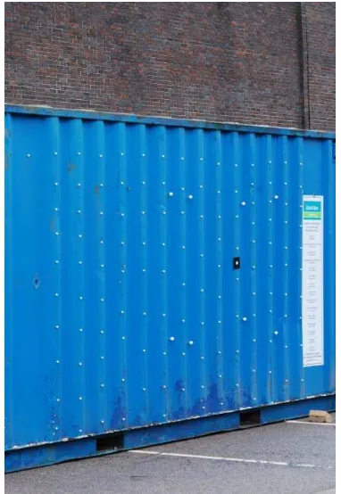
Geometric camera calibration was conducted through self-calibration after the field season, using a test field area of approximate size of 6 m2. This consisted of a steel wall and 132 magnetic spherical white targets (Figure 4). These targets were constructed using a precision spherical plastic ball with a magnetic component, which allows quick placement on the
wall. The positions of the targets were not known precisely, but were distributed evenly across the surface of the test field. 15 convergent images were acquired from five camera stations located 3 meters from the test field. At each station, the camera was rotated around its optical axis by 0º, 90º and -90º. Photographs were acquired at the minimum zoom setting with the autofocus feature activated. This equates to the default camera settings after the camera was "switched on", and was identical to the settings used during fieldwork. All image point measurement ("Automarking") and self-calibration were executed using the Photomodeller Scanner software and an overall point marking residual of 0.169 pixels and an overall RMS Vector Length of 0.3 mm was obtained. A focal length (6.256 mm) and principal point position (3.798 mm, 2.731 mm) were recovered, with a standard deviation lower than 0.8 microns. The first radial distortion parameter (4.036x10⁻³) was recovered with a standard deviation of 1.6x10⁻⁵. The second radial distortion parameter (-7.267x10⁻⁵) was recovered with a standard deviation of 9.2x10⁻⁷. Decentering parameters P1 (-1.997x10⁻⁴) and P2 (-2.393x10⁻⁴) were recovered with standard deviations of 5.3x10⁻⁶ and 5.3x10⁻⁶ respectively.
This calibration set was judged suitable for processing of the imagery, assuming that camera stability was sufficient for the task of generating ice surface representations.
Figure 2. One of the 4 m2 area photographs
Figure 3. One of the 1 m2 area photographs
3.3 Photogrammetric processing
Photogrammetric processing of stereo pairs was done with the automatic matching tool "Smartpoints", initially introduced into Photomodeller Scanner in the autumn of 2011. This tool automatically marks and references points using natural features, then orients and processes the photos to provide fully automatic project set up and relative orientation. The absolute orientation and scaling of the photogrammetric survey was performed by manually marking points on the pole (origin) and marks on the ropes and enforcing external and assumed geometric constraints. This entailed defining a coordinate system in which the X axis is the horizontal axis represented in Figure 5 and Y axis was approximately horizontal and perpendicular. The reference pole defines the origin (0, 0) and area of interest is in the second quadrant.
After obtaining the absolute positions and orientations of stereo-pairs the data-processing continued in the normal sequence and involved generating point clouds using the automatic tool "create dense surface". This was achieved at a nominal point density of 4 mm and was surprisingly successful at certain scales, particularly when considering the reflective properties of the ice (Figure 5, Section 4.1).
Figure 4. Field calibration metallic wall
3.4 Points clouds post-processing
From the data obtained in the point clouds, a regular grid of 251x251 nodes (4 mm x 4 mm) was generated. Each node height was calculated through Kriging, an interpolation method based on regression against observed z values of surrounding data points. Although Kriging is considered an optimal interpolator in the sense that the estimates are unbiased and have known minimum variances, no major differences can be expected when compared with other interpolation methods, given the high density and the large number of points available in the point clouds.
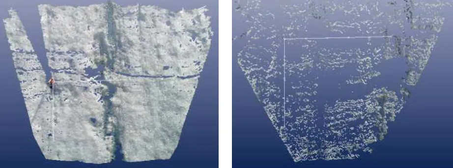
Figure 5. Top view of the 1 m2 (left) and 4 m2 (right) point clouds.
4. RESULTS AND DISCUSSION
The derivation of point clouds covering a common area, acquired using imagery of the same date/time, and at three different scales, provided an opportunity to assess the quality of surface representation. This would also allow the performance of the overall methodology, the automatic processes (relative orientation and DEM extraction) and absolute orientation and scaling procedures to be evaluated also. Four different point clouds were obtained using 4 different pairs of the same 1 m2 area. Unfortunately, no independent check data of sufficient quality could be obtained in the hostile environment to enable true accuracy to be determined. An attempt was made to determine check profiles using conventional taping but this was judged to be too poor for any rigorous accuracy assessment.
4.1 Points clouds
As expected, very different results were obtained depending on the image scale. For the 25 m2 area images, DEM generation results were very poor, with only a few tens of points derived. In direct contrast, the 1 m2 area images generated hundreds of thousands points (Figure 5). Images representing the 4 m2 plots showed intermediate results, with tens of thousands of points measured (Figure 5). Although the number of points remains high, the large holes create a poor characterisation of the glacial surface and was therefore discarded for the remainder of this study.
The wide range of behaviour exhibited by the different scales can be explained by identifying 3 different aspects. First, the varying obliquity associated with the different scales. A shallow viewing angle creates larger areas of shade or "dead ground" behind the ridges that are apparent (Figure 2). Second, the texture obtained in the three areas is very different because the cryoconite/pixel and rugosity/pixel size ratio varies greatly. Lastly, in the 25 m2 area, the appearance of very dark hills in the distance (Figure 1) reduces the available dynamic range of pixel values. The pixels representing the glacier appear as a homogeneous white surface without sufficient variation to represent surface texture and with luminosity values close to overexposure.
In the 1 m2 area stereo-pairs, the high convergence over the ground (Figure 6) and the good texture obtained due to the cryoconite/pixel and rugosity/pixel ratio size ratio allows derivation of very dense point clouds. Figure 7 shows the relation between the number of points obtained as a function of
DEM density.
In the 1 m2 area, a pixel represents 7 mm on the ground. Although the interpolated sub-pixel algorithms allow DEM generation at even higher resolutions, at a certain point density of interpolated results do not provide any additional surface information. It was decided that a 4 mm surface resolution represented an optimum density to obtain a surface representation using the least number of points possible. This density of points was adopted for the four point clouds used for further analysis.
Figure 6. Data capturing setup for 1 m2 area, showing a 52º of convergence.
Figure 7. Number of points in the cloud as function of DEM density.
4.2 DEM consistency
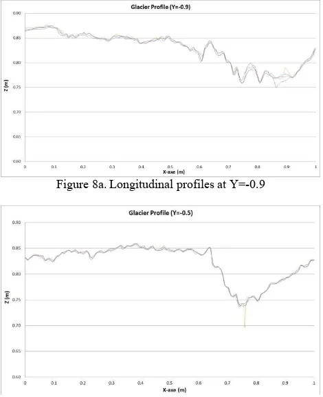
Figure 8 shows the different longitudinal profiles oriented along the x-axis direction (perpendicular to glacier slope) and representing the surface glacier within the 1 m2 area of interest
obtained. Figure 8a represents the profile obtained for Y=-0.9, Figure 8b from Y=-0.5 and Figure 8c generated from a Y coordinate equal to -0.1.
As can be observed, most of the profiles are coincident except within the small-scale supra-glacial channels or supra-glacial rills. These low areas correspond to holes in the cloud, i.e. shadow areas where there is no clear 3D information captured.
Figure 8a. Longitudinal profiles at Y=-0.9
Figure 8b. Longitudinal profiles at Y=-0.5
Figure 8c. Longitudinal profiles at Y=-0.1
Further analysis focused on an area free of holes/dead ground, (0<X<0.5 and -1<Y<0). In this region the difference was calculated between one reference cloud points and the other three, for each of the 31,626 nodes. The resulting data from the three difference models was combined and plotted in a single histogram (Figure 9). A best fit normal distribution profile was determined, representing a standard deviation of just 2.3 mm. This demonstrates an excellent internal accuracy which surely shows that the derived data is fit for generating surface roughness parameters for many glaciological applications.
Figure 9. Differences between the 4 points clouds.
It´s difficult to find another measurement instrument or technique so suitable to measure glacier surface roughness with sub-centimeter precision. Manual micro-topographic surveying can be time consuming, may lack the necessary vertical resolution and/or is disruptive to the surface. Airborne laser scanning or digital photogrammetry are only suitable for larger-scale cryospheric applications. Terrestrial laser scanning (TLS) has been successfully trialled for snow and glacier surfaces but the size and weight of the equipment, combined with the complexity of the data processing, currently prevents the technology from immediately being used extensively in glaciological field work (Kerr et al., 2009). Lastly, image-based measurements using a thin black plate inserted into snow or ice reports good horizontal and vertical resolutions. However, this technique is limiting as it is based on singular profiles which have be defined during fieldwork.
5. CONCLUSIONS
Many studies related to glacier melt processes require precise knowledge of the roughness of the surface of the glacier at levels of detail not attainable by conventional techniques like airborne laser scanner or aerial photogrammetry. This paper demonstrates that close-range photogrammetry using a consumer grade digital camera allows detailed DEM extraction and offers important advantages over terrestrial laser scanning. First, the necessary equipment in the field is very simple; a standard camera, a polyethylene pole and some rope. Secondly, data collection involves simply capturing imagery. This is a "quasi-instantaneous" procedure which enables high productivity, an important factor given the difficult environmental conditions encountered when conducting field-work on a glacier.
The convergence of photos, the resolution of the camera and the extent of shadows areas remain a limiting constraint in generating good DEMs. The height of an operator above the ground is sufficient to survey small areas of 1 m2, but for larger areas results have been poor. It is suggested that for a 28 mm focal length camera, the viewpoint needs to be raised by approximately 60 cm to survey an area of 4 m2. An additional camera height of 120 cm is necessary to obtain appropriate geometry for a surface area of 9 m2. The camera resolution is the second important constraint. For a study area of 1 m2 and a camera with 5 megapixels, precisions have been better than 3 mm. If results are extrapolated and considering the current state of the art in standard camera resolution (18 Megapixels), a 4.5 mm precision would be achieved in 4 m2 study areas and 6 mm for 9 m2 areas. A single stereo-pair is perhaps insufficient to
obtain 3D data within supra-glacial rills, because in each of the photographs one of the supra-glacial channel slopes is not visible. Results could be improved either by taking an additional centered photograph or two additional side photos.
This study has demonstrated that digital close-range photogrammetry has proven to be a useful technique to reconstruct the glacier's surface with sub-centimeter precision. Such an approach may prove to be useful a method by which the relationship between cryoconite and ice surface properties can be explored over either space or time.
6. REFERENCES
Arnold, N.S., Rees, W.G., 2004. Self-similarity in glacier surface characteristics. Journal of Glaciology, 49(167), pp. 547–554.
Baltsavias, E. P., Favey, E., Bauder, A., Boesch, H., Pateraki, M., 2001. Digital surface modelling by airborne laser scanning and digital photogrammetry for glacier monitoring, The Photogrammetric Record, 17(98), pp. 243–273.
Bøggild, C.E., Brandt, R.E., Brown, K.J., Warren, S.G., 2010. The ablation zone in northeast Greenland: ice types, albedos, and impurities. Journal of Glaciology, 56(195), pp. 101–113.
Brock, B., Willis, I.C., Sharp, M.J., 2006. Measurement and parameterization of aerodynamic roughness length variations at Haut Glacier d'Arolla, Switzerland. Journal of Glaciology, 52(177), pp. 281–297.
Fassnacht, S.R., Williams, M.W., Corrao M.V., 2009. Changes in the surface roughness of snow from millimetre to metre scales. Ecological Complexity, 6(3), pp. 221–22.
Fassnacht, S.R., Stednick, J.D., Deems, J.S., Corrao, M.V., 2010. Metrics for assessing snow surface roughness from Digital imagery. Water Resources Research, 46(4), art. no. W00D31.
Fox, A.J., Gooch, M.J., 2001. Automatic DEM generation for Antarctic terrain. The Photogrammetric Record, 17(98), pp. 275–290.
Hodson, A., Cameron, K., Bøggild, C., Irvine-Fynn, T., Langford, H., Pearce, D., Banwart, S., 2010. The structure, biogeochemistry and formation of cryoconite aggregates upon an Arctic valley glacier; Longyearbreen, Svalbard. Journal of Glaciology, 56(195), pp. 349–362.
Höfle, B., Geist, T., Rutzingera, M., Pfeife, N., 2007. Glacier surface segmentation using airborne laser scanning point cloud and intensity data. IAPRS, Espoo, Finland, Vol. XXXVI, pp. 195–200.
Hopkinson C., 2004. Place Glacier terrain modelling and 3D laser imaging. Geological Survey of Canada, Report TSD051603X, 22pp.
Hopkinson, C., Demuth, M.N., 2006. Using airborne lidar to assess the influence of glacier downwasting on water resources in the Canadian Rocky Mountains. Canadian Journal of Remote Sensing, 32(2), pp. 212–222.
Irvine-Fynn, T.D.I., Sanz-Ablanedo, E., Rutter, N., Chandler, J.H. In prep. Measuring glazier roughness using close range digital photogrammetry. Journal of Glaciology.
Kaasalainen, S., Kaartinen, H., Kukko, A., Anttila, K., Krooks, A., 2011. Brief communication "application of mobile laser scanning in snow cover profiling". Cryosphere, 5(1), pp. 135– 138.
Kaufmann, V., Ladstädter, R., 2008. Application of terrestrial photogrammetry for Glacier monitoring in alpine environments. The International Archives of the Photogrammetry, Remote Sensing and Spatial Information Science, Beijing, China, Vol. XXXVII, Part B8, pp. 813–818.
Kerr, T., Owens, I., Rack, W., Gardner, R., 2009. Using ground-based laser scanning to monitor surface change on the Rolleston Glacier, New Zealand. Journal of Hydrology (NZ), 48(2), pp. 59–72.
Kirby, R.P., 1991. Measurement of surface roughness in desert terrain by close range photogrammetry. The Photogrammetric Record, 13(78), pp. 855–875.
Nolin, A.W., Fetterer, F.M., Scambos, T.A., 2002. Surface roughness characterizations of sea ice and ice sheets: Case studies with MISR data. IEEE Transactions on Geoscience and Remote Sensing, 40 (7), pp. 1605–1615.
Rees, W.G., 1998. Correspondence. A rapid method for measuring snow surface profiles. Journal of Glaciology, 44(148), pp. 674–675.
Rees, W.G., Arnold, N.S., 2006. Scale-dependent roughness of a glacier surface: implications for radar backscatter and aerodynamic roughness modelling. Journal of Glaciology, 52(177), pp. 214–222.
Rieke-Zapp D.H., Nearing, M.A., 2005. Digital close range photogrammetry for measurement of soil erosion. The Photogrammetric Record, 20(109), pp. 69–87.
Taconet, O., Ciarletti, V., 2007. Estimating soil roughness indices on a ridge-and-furrow surface using stereo photogrammetry. Soil and Tillage Research, 93(1), pp. 64–76.
Takeuchi, N., 2002. Optical characteristics of cryoconite (surface dust) on glaciers: the relationship between light absorbency and the property of organic matter contained in the cryoconite. Annals of Glaciology, 34(1), pp. 409-414.
Takeuchi, N., Nishiyama, H., Li Z., 2010. Structure and formation process of cryoconite granules on Ürümqi glacier No. 1, Tien Shan, China. Annals of Glaciology, 51(56), pp. 9–14.
7. ACKNOWLEDGEMENTS
ESA acknowledges Spanish Ministerio de Educación y Ciencia, Program “José Castillejo 2010-2011”.
TIF acknowledges NERC Standard Grant NE/G006253/1 (PI: AJ Hodson, University of Sheffield), and support from the Climate Change Consortium of Wales (C3W). Logistical support in Svalbard was provided by Nick Cox (NERC Arctic Research Station), and field assistants Aga Nowak-Zwierz and Jon Bridge (University of Sheffield).