A CONVOLUTIONAL NETWORK FOR SEMANTIC FACADE SEGMENTATION AND
INTERPRETATION
Matthias Schmitz, Helmut Mayer
Institute for Applied Computer Science Bundeswehr University Munich
Werner-Heisenberg-Weg 39, 85577 Neubiberg, Germany [email protected], [email protected]
Commission III, WG III/4
KEY WORDS:Convolutional Network, Deep Learning, Facade Interpretation, Object Detection, Segmentation
ABSTRACT:
In this paper we present an approach for semantic interpretation of facade images based on a Convolutional Network. Our network processes the input images in a fully convolutional way and generates pixel-wise predictions. We show that there is no need for large datasets to train the network when transfer learning is employed, i. e., a part of an already existing network is used and fine-tuned, and when the available data is augmented by using deformed patches of the images for training. The network is trained end-to-end with patches of the images and each patch is augmented independently. To undo the downsampling for the classification, we add deconvolutional layers to the network. Outputs of different layers of the network are combined to achieve more precise pixel-wise predictions. We demonstrate the potential of our network based on results for the eTRIMS (Korˇc and F¨orstner, 2009) dataset reduced to facades.
1 INTRODUCTION
Deep Learning and especially Convolutional Networks (ConvNets) are gaining more and more interest in recent years. One of their first applications has been document recogni-tion (LeCun et al., 1998). Others are image classificarecogni-tion, where a single label is assigned to a whole image (Krizhevsky et al., 2012, Simonyan and Zisserman, 2014, Szegedy et al., 2015) or semantic segmentation with Fully Convolutional Networks (Long et al., 2015). When only few data is available, transfer learning can be a good choice to fine-tune an already learned network (Zeiler and Fergus, 2014, Donahue et al., 2014).
With the growing need for three-dimensional (3D) city-models in cultural heritage, town planing, tourism, etc., their automatic generation is an ongoing research topic. Semantic interpretation of facades, especially the detection of doors and windows is necessary for level-of-detail (LOD) 3 building models (Kolbe et al., 2005). There are different approaches for this: Some authors use 3D point clouds for geometric interpretation (Nguatem et al., 2014) or learn grammars from labeled facade images and use them for parsing (Martinovic and Van Gool, 2013). Others search for repetitive patterns on two-dimensional (2D) input images to segment individual facades (Wendel et al., 2010) or try to find windows with the help of implicit shape models (Reznik and Mayer, 2008).
With regard to both the growing need for semantic build-ing models as well as the developbuild-ing field of Deep Learnbuild-ing, we present in this paper an approach based on ConvNets to segment and classify facade-elements in images.
In the following section we summarize previous work. The basic ideas of ConvNets and some of their advantages over other methods are presented in Section 3. Section 4 deals with our ConvNet structure and Section 4.1 with the way it is trained. Validation of our method follows in Section 4.2. The paper ends with the conclusion.
2 RELATED WORK
With an optimized GPU (graphics processing unit) implementa-tion of 2D convoluimplementa-tions and other ConvNet-specific operaimplementa-tions, (Krizhevsky et al., 2012) made available a basis for efficient Deep Learning and ConvNets. They also introduced features, like the ReLU nonlinearity or the overlapping pooling operation, which often lead to better results and/or faster training. Another important part of their work is the reduction of overfitting by augmentation of the training data and the inclusion ofdropout into the network. These techniques are used in our work and will be presented in Section 3. Other work such as GoogLeNet (Simonyan and Zisserman, 2014) and VGG net (Szegedy et al., 2015) has been inspired by (Krizhevsky et al., 2012).
(Long et al., 2015) introduced a fully convolutional approach for semantic segmentation. They use the networks introduced above, which were trained for classification, and adapted them for pixel-wise prediction. Particularly, the networks were converted into fully convolutional versions and then fine-tuned with and for new data. For better results, (Long et al., 2015) combined the output of deep layers, which are coarser, but contain more information, with shallow and thus more detailed layers.
(Hariharan et al., 2015) have shown that combining coarse and fine layers is important for pixel-wise image segmentation. The deepest layers contain most of the semantic information, but are not precisely located in the spatial domain. Shallow layers, on the other hand, are very precisely localized in in the spatial domain (e .g., position of edges), but contain less semantics. By combining all features into ahypercolumn, the resulting vector contains information for both, semantics and location.
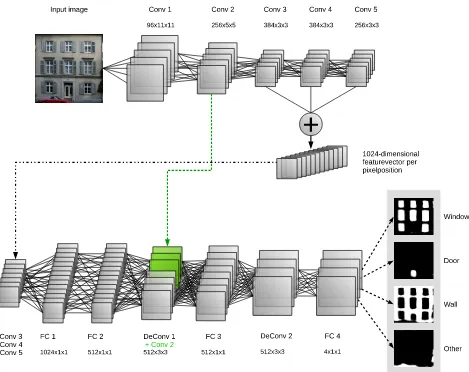
Figure 1: Employed ConvNet with convolutional layers (Conv), fully convolutional layers (FC) and deconvolutional layers (DeConv). The layers are described by the number of resulting feature maps and the size of the (de)convolution kernel. Layers Conv 3, 4, and 5 are concatenated to 1024 feature maps. To the feature maps of DeConv 1 the feature maps of Conv 2 (green part) are concatenated. Finally, a softmax function computes the probabilities of all classes at each pixel position. Probabilities are coded from black (low) to white (high).
input image. The result of the deepest layer is upsampled by deconvolutions. The authors call the convolutional side of their network contracting path, the deconvolutional side expansive path. Features from the contracting path are concatenated with features from the expansive path. Thus, the deepest layers contain both, spatial and semantic information. Training is done end-to-end with augmented patches of complete images, so there was much more training data than images. Data augmentation is done by deformation of the training data.
In the field of facade interpretation from images, (Reznik and Mayer, 2008) search for windows using an implicit shape model (Leibe and Schiele, 2004). They find corners of windows by matching patches at points of interest to patches from the training data via cross correlation and employ them to generate hypotheses for window outlines. To further improve the recogni-tion rate, the detected windows are arranged in rows, columns or grids.
( ˇCech and ˇS´ara, 2009) employ pixel intensities for window detection as well as a Markov Random Field (MRF) with asym-metric pair wise compatibilities and a shape-based language. The detection of regular window patterns has been improved by
(Tyleˇcek and ˇS´ara, 2012) by guiding it with a stochastic grammar with pair-wise attribute constraints. In (Tyleˇcek and ˇS´ara, 2013), additionally a data-dependent topology of spatial templates has been introduced.
(Simon et al., 2011) segment facades into windows and doors as well as a couple of other objects. The approach has been tested on facades with many repetitions and regularities which can be described well by only six grammar rules. A pixel-wise random forest is used to find evidence when selecting grammar rules. While shape priors are integrated, the outline of the objects is not considered leading to only an approximation of the geometry.
3 CONVOLUTIONAL NETWORKS
ConvNets are biologically inspired Machine Learning algo-rithms, which are based on classical Artificial Neural Networks (ANN) or Multilayer Perceptrons (MLP). In an MLP, a given in-put is mapped onto the outin-put over two or more layers of nodes (neurons). Each node of one layer has a weighted connection to each node of the subsequent layer. The output of a single neu-ron is computed via an activation function over the sum of its weighted inputs (plus some bias) (see Equation 1)
yl+1
Typically, training of the MLP is done in a supervised manner by means of the backpropagation algorithm: Training examples are pairs of input and label. The input is processed by the network and the networks output is compared to the given label. An error-function (e. g., euclidean distance) computes the output error and this error is propagated back through the network. Depending on the error, the network weights are changed. This procedure is repeated multiple times with all training examples.
In contrast to the completely connected layers in MLP, the connections between two subsequent layers in a ConvNet are often locally restricted, but repeated over the input. This effect is comparable to convolutions, whose kernels are learned by the training algorithm. Another interpretation is, that each layer of a ConvNet extracts different features from the preceding layer. In shallow (fine) layers, i. e., layers at the top, the extracted features are simple like edges or color-patches in the input image. For deeper (coarse) layers, features become more complicated, e. g., small objects, object parts or patches.
In addition to the convolutional layers, many different lay-ers and techniques have been developed in recent years, e. g., (Krizhevsky et al., 2012). We shortly introduce those we use in our configuration:
Feature map Often, the output of a kernel is called a feature map.
Convolution This is the most important layer type of a Con-vNet. Weighted connections are locally restricted, but re-peated over the image or feature map. The resulting feature maps are equal to a convolution with the (learned) kernels. Sometimes a step size (in the context of ConvNets called stride) is given, that defines the number of pixels between two convolutions or rather at what position the next repeti-tion of the weights is applied.
Deconvolution The inverse function of a convolution. A single pixel of a layer is split into multiple pixels of the subsequent layer. This is also done with learned weights. Analog to the Convolution layer, a Deconvolution layer can have a stride.
Fully connected Like in a MLP each node of one layer is con-nected to each node of the next layer.
ReLU The Rectified Linear Unit (ReLU) is used as activation function. It is defined as:
f(x) = max(0, x).
Pooling A pooling layer maps two or more pixels to a single pixel. For example, pooling can be done by averaging or taking the maximum value.
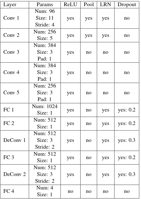
Layer Params ReLU Pool LRN Dropout
Conv 1
Table 1: Layer configurations of the employed network (cf. Fig-ure 1). The first two columns give the name of the layer and the number of feature maps as well as the size of the (de)convolution kernels. In the following columns we specify if a layer is fol-lowed by a non-linearity (ReLU), a pooling layer (Pool), a local response normalization layer (LRN) or a dropout layer. For the dropout, also the probability for the dropout of each node is given.
LRN Local Response Normalization (LRN) is comparable to lateral inhibition in biological context. If the output of one kernel is big, it will suppress the outputs of the neighboring kernels. This leads to diverging kernels, i. e., neighboring kernels are clearly different.
Dropout When dropout is used, the output of a neuron will be zero with a given probability while learning. The effect is, that the architecture of the network is different for each it-eration, but the shared weights are always the same. The result is a more stable ConvNet.
Augmentation Large amounts of data are essential for training robust networks. Because it is not always possible or afford-able to collect more data, additional realistic data is gener-ated by augmenting the available data, e. g., by scaling, ro-tation, or adding noise to the gray or color values.
4 A CONVNET FOR FACADES
followed by two fully convolutional layers, which can be seen as a pre-classification.
Because the output of layers three, four and five is much smaller than the input, we add deconvolutional layers. After the first deconvolution, we reintroduce more shallow features by concatenating the output-feature maps with the output of layer two, to get more precisely located results. Both deconvolutional layers are followed by a fully convolutional layer, which also leads to more precise results. The output of the last fully connected layer and, therefore, of the ConvNet as a whole, is a four-dimensional vector of probabilities, that the output pixel belongs to one of the four classes building, door, window, and other. At runtime, we use a softmax-layer on top of it. The softmax-function is defined as following:
σ(xi) =
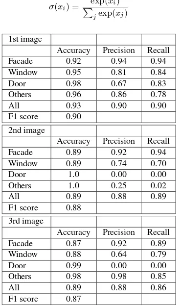
Table 2: Accuracy, Precision and Recall for best results (see Fig-ure 2)
4.1 Training
As this paper is concerned with facade interpretation, we use the eTRIMS (Korˇc and F¨orstner, 2009) images and labels for training and validation. For our specific application they are manually preprocessed: Individual facades are cut out and roughly recti-fied. Due to the fact that ConvNets are able to learn deviations, i. e., are very robust against small perturbations, perfect data is not necessary. Facades are classified intofacade, door, and window. All other labels of the eTRIMS data are combined into the classother. Although the original eTRIMS dataset contains eight labels, namely building, car, door, pavement, road, sky, vegetation, andwindow, there are two reasons to combine five classes: First, we want to segment and classify facade-objects and some of the classes do not belong to them. Second, because we cut out the facades from the original images, in most cases there are very few pixels that belong to some of the classes. Thus,
1st image
Table 3: Accuracy, Precision and Recall for worst results (see Figure 3)
Table 4: Overall Accuracy, Precision and Recall
the available amount of data for training these classes is much too small. Patches of size131×131pixels are extracted from the images. Corresponding patches are extracted from the label images and scaled down to the size of the output (23×23pixels).
To increase robustness of the learned model, we augment the available data in two ways: First, the extracted patches are randomly mirrored horizontally. Second, we also artificially enlarge the dataset by scaling the extracted image- and label-regions by an independent random factor in both dimensions and rescaling it to131×131pixels. Using patches lead to much more training data than images and augmenting them increases variation. The size of131×131pixels is chosen to speed up the training time while at the same time avoiding too much correlation for the training data.
Training is done by backpropagation with stochastic gradi-ent descgradi-ent. As error-function we used cross-entropy after computing the softmax for each pixel of the last layer. Cross-entropy is defined as:
Training the network took about 8 hours on an NVIDIA Quadro K5200 using the Caffe implementation. (Jia et al., 2014).
4.2 Validation and Evaluation
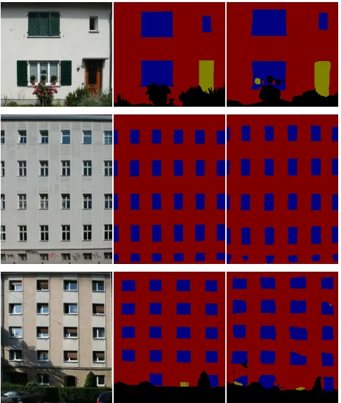
For validation, the eTRIMS dataset was divided into six subsets of 10 images. This is the basis for six-fold cross-validation, i. e., we trained six networks, each with 50 training images and tested them on the remaining 10 images. Figure 2 and Table 2 give results for the three best images (concerning the F1 score) and Figure 3 and Table 3 for the three worst results, respectively.
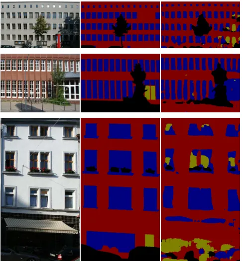
The first column of Figures 2 and 3 presents the original image. The second column shows the ground-truth label image and the result of our network is given in the third column. The colors in the label images define the different classes: Red for facades, blue forwindows, yellow fordoors, and the classother is displayed in black.
For evaluation, we used the following statistical measures:
• Accuracy: T P+T N ALL
• Precision (Exactness, Correctness): T P T P+F P
• Recall (Completeness): T P T P+F N
• F1 score (harmonic mean of precision and recall): 2T P
2T P+F P+F N
with true positives TP, false positives FP, true negatives TN, and false negatives FN for each class.
A weighted average value over all four classes is computed w. r. t. the amount of ground-truth pixels per class (cf. Table 4). It shows that windows and objects of the classother, especially vegetation (potted plants in front of the window in the first row of Figure 2) are well recognized. Shadows can lead to problems as can be seen in the top row of Figure 3, where windows are classified as doors and structured shadows on the facade asother. Doors made of glass or containing glass elements or windows are often classified as windows. In most cases this is not surprising. For example the doors in the second row of Figure 3 have the same structure and texture as the surrounding windows.
Our network is able to recognize windows that are partially occluded, as can be seen in the first and third row of Figure 2 and all examples of Figure 3.
5 CONCLUSION
In this paper we have presented a method for semantic facade-segmentation based on a ConvNet. By using parts of already-trained networks and fine-tuning them and by employing augmented patches of images, no big datasets are necessary to obtain good results in a reasonable training time. We trained and tested our network on subsets of images limited to the facades of the eTRIMS dataset. The overall results achieve an F1 score of 82% for the four classes facade, door, window, and other.
For future work, we want to analyze the contributions of the various parts of our network for the results as well as limitations arising from the network as well as limited training data.
REFERENCES
ˇ
Cech, J. and ˇS´ara, R., 2009. Languages for Constrained Binary Segmentation Based on Maximum Aposteriori Probability La-beling. International Journal of Imaging and Technology 19(2), pp. 69–79.
Donahue, J., Jia, Y., Vinyals, O., Hoffman, J., Zhang, N., Tzeng, E. and Darrell, T., 2014. DeCAF: A Deep Convolutional Acti-vation Feature for Generic Visual Recognition. In: International Conference on Machine Learning, pp. 647–655.
Green, P., 1995. Reversible Jump Markov Chain Monte Carlo Computation and Bayesian Model Determination. Biometrika 82(4), pp. 711–732.
Hariharan, B., Arbel´aez, P., Girshick, R. and Malik, J., 2015. Hypercolumns for Object Segmentation and Fine-Grained Local-ization. In: IEEE Conference on Computer Vision and Pattern Recognition, pp. 447–456.
Jia, Y., Shelhamer, E., Donahue, J., Karayev, S., Long, J., Gir-shick, R., Guadarrama, S. and Darrell, T., 2014. Caffe: Convo-lutional Architecture for Fast Feature Embedding. arXiv preprint arXiv:1408.5093.
Kolbe, T. H., Gr¨oger, G. and Pl¨umer, L., 2005. CityGML: In-teroperable Access to 3D City Models. In: P. van Oosterom, S. Zlatanova and E. M. Fendel (eds), Geo-information for Disas-ter Management, Springer Berlin Heidelberg, pp. 883–899.
Korˇc, F. and F¨orstner, W., 2009. eTRIMS Image Database for Interpreting Images of Man-Made Scenes. Technical Report TR-IGG-P-2009-01.
Krizhevsky, A., Sutskever, I. and Hinton, G. E., 2012. Ima-genet Classification with Deep Convolutional Neural Networks. In: Advances in Neural Information Processing Systems 25, pp. 1097–1105.
LeCun, Y., Bottou, L., Bengio, Y. and Haffner, P., 1998. Gradient-based Learning applied to Document Recognition. Proceedings of the IEEE 86(11), pp. 2278–2324.
Leibe, B. and Schiele, B., 2004. Combined Object Categorization and Segmentation with an Implicit Shape Model. In: ECCV’04 Workshop on Statistical Learning in Computer Vision, pp. 1–16.
Long, J., Shelhamer, E. and Darrell, T., 2015. Fully Convolu-tional Networks for Semantic Segmentation. In: IEEE Confer-ence on Computer Vision and Pattern Recognition, pp. 3431– 3440.
Martinovic, A. and Van Gool, L., 2013. Bayesian Grammar Learning for Inverse Procedural Modeling. In: IEEE Conference on Computer Vision and Pattern Recognition, pp. 201–208.
Nguatem, W., Drauschke, M. and Mayer, H., 2014. Localiza-tion of Windows and Doors in 3D Point Clouds of Facades. In: ISPRS Annals of Photogrammetry, Remote Sensing and Spatial Information Sciences, Vol. II-3, pp. 87–94.
Reznik, S. and Mayer, H., 2008. Implicit Shape Models, Self Diagnosis, and Model Selection for 3D Facade Inter-pretation. Photogrammetrie, Fernerkundung, Geoinformation 2008(3), pp. 187–196.
Figure 2: This figure presents the three results with the best F1 score. The original image is shown in the first column, followed by the ground-truth label image. The result of our network is shown in the last column. The colors of the label images define the different classes: red – facade, blue – window, yellow – door, and black – other.
Simon, L., Teboul, O., Koutsourakis, P. and Paragios, N., 2011. Random Exploration of the Procedural Space for Single-View 3D Modeling of Buildings. International Journal of Computer Vision 93(2), pp. 253–271.
Simonyan, K. and Zisserman, A., 2014. Very Deep
Convo-lutional Networks for Large-Scale Image Recognition. arXiv preprint arXiv:1409.1556.
Figure 3: The three results with the worst F1 scores. The columns and the label colors are the same as in Figure 2.
Tyleˇcek, R. and ˇS´ara, R., 2012. Stochastic Recognition of Regu-lar Structures in Facade Images. IPSJ Transactions on Computer Vision and Applications 4, pp. 63–70.
Tyleˇcek, R. and ˇS´ara, R., 2013. Spatial Pattern Templates for Recognition of Objects with Regular Structure. In: J. Weickert, M. Hein and B. Schiele (eds), 35th German Conference on Pat-tern Recognition, LNCS, Vol. 8142, Springer Berlin Heidelberg, pp. 364–374.
Wendel, A., Donoser, M. and Bischof, H., 2010. Unsupervised Facade Segmentation Using Repetitive Patterns. In: M. Goesele, S. Roth, A. Kuijper, B. Schiele and K. Schindler (eds), Pattern
Recognition: 32nd DAGM Symposium, Springer Berlin Heidel-berg, pp. 51–60.