END-TO-END DEPTH FROM MOTION WITH STABILIZED MONOCULAR VIDEOS
C. Pinarda,b∗, L. Chevalleya, A. Manzanerab, D. Filliatb
aParrot, Paris, France - (clement.pinard, laure.chevalley)@parrot.com b
U2IS, ENSTA ParisTech, Universite Paris-Saclay, Palaiseau, France - (antoine.manzanera, david.filliat)@ensta-paristech.fr
KEY WORDS:Dataset, Navigation, Monocular, Depth from Motion, End-to-end, Deep Learning
ABSTRACT:
We propose a depth map inference system from monocular videos based on a novel dataset for navigation that mimics aerial footage from gimbal stabilized monocular camera in rigid scenes. Unlike most navigation datasets, the lack of rotation implies an easier structure from motion problem which can be leveraged for different kinds of tasks such as depth inference and obstacle avoidance. We also propose an architecture for end-to-end depth inference with a fully convolutional network. Results show that although tied to camera inner parameters, the problem is locally solvable and leads to good quality depth prediction.
1. INTRODUCTION
Scene understanding from vision is a core problem for autonomous vehicles and for UAVs in particular. In this paper we are specifi-cally interested in computing the depth of each pixel from a pair of consecutive images captured by a camera. We assume our camera’s velocity (and thus displacement between two frames) is known, as most UAV flight systems include a speed estimator, allowing to settle the scale invariance ambiguity.
Solving this problem could be beneficial for applying depth-based sense and avoid algorithms for lightweight embedded systems that only have a monocular camera and cannot directly provide a RGB-D image. This could allow such devices to go without heavy or power expensive dedicated devices such as ToF cam-era, LiDar or Infra Red emitter/receiver (Hitomi et al., 2015) that would greatly lower autonomy. In addition, many RGBD sen-sors are unable to operate under sunlight (e.g. IR and ToF), and most of them suffer from range limitations and can be inefficient in case we need long-range trajectory planning (Hadsell et al., 2009). The faster an UAV is, the longer the range we will need to efficiently avoid obstacles. Unlike RGB-D sensors, depth from motion is robust to high speeds since it will be normalized by the displacement between two frames. Given the difficulty of the task, several learning approaches have been proposed to solve it.
A large number of datasets has been developed in order to pro-pose supervised learning and validation for fundamental vision tasks, such as optical flow (Geiger et al., 2012,Dosovitskiy et al., 2015, Weinzaepfel et al., 2013) stereo disparity and even 3D scene flow (Menze and Geiger, 2015,N.Mayer et al., 2016). These different measures can help figure up scene structure and camera motion, but they remain low-level in terms of abstrac-tion. End-to-end learning of a certain value such as three dimen-sional geometry may be hard to compute on a totally unrestricted monocular camera movement.
We focus on RGB-D datasets that would allow supervised learn-ing of depth. RGB pairs (preferably with the correspondlearn-ing dis-placement) being the input, and D the desired output. It turns out that today, for learning depth from video, the choice among existing RGB-D datasets is either unrestricted w.r.t. ego-motion
∗Corresponding author
a) b) c)
Figure 1. Camera stabilization can be done via a) mechanic gimbal or b) dynamic cropping from fish-eye camera, for drones
or c) hand-held cameras
(Firman, 2016,Sturm et al., 2012), or based on stereo vision, equivalent to lateral movement (Geiger et al., 2012,Scharstein and Szeliski, 2002).
We thus propose a new dataset, described Part 3, which aims at proposing a bridge between the two by assuming that rotation is canceled on the footage that contains only random translations.
This assumption about videos without rotation appears realistic for two reasons:
• hardware rotation compensation is mainly a solved problem, even for consumer products, with IMU-stabilized cameras on consumer drones or hand-held steady-cam (Fig 1).
• this movement is somewhat related to human vision and vestibulo-ocular reflex (VOR) (De N´o, 1933). Our eyes ori-entation is not only induced by head rotation, our inner ear among other biological sensors allows us to compensate par-asite rotation when looking at a particular direction.
Assuming only translations allows to dramatically simplify links between optical flow and depth, and leverage much simpler com-putation. The main benefit being the camera movement’s dimen-sionality, reduced from 6 (translation and rotation) to 3 (only translation). However, as discussed in Part 4, depth is not com-puted as simply as with stereo vision and requires being able to compute higher abstractions to avoid a possible indeterminate form, especially for forward movements.
2. RELATED WORK 2.1 Monocular vision based sense and avoid
Sense and avoid problems are mostly approached using a ded-icated sensor for 3D analysis. However, some works have been done trying to leverage Optical flow from Monocular camera (Souhila and Karim, 2007,Zingg et al., 2010). They highlight the diffi-culty of estimating depth solely with flow, especially when the camera is pointed toward movement. One can note that rota-tion compensarota-tion was already used with fish-eye camera in or-der to have a more direct link between flow and depth. Another work (Coombs et al., 1998) also demonstrated that basic obstacle avoidance could be achieved in cluttered environments such as a closed room.
Some interesting work concerning obstacle avoidance from Monoc-ular camera (LeCun et al., 2005,Hadsell et al., 2009,Michels et al., 2005) showed that single frame analysis can be more efficient than depth from stereo for path planning. However, these works were not applied on UAV, on which depth cannot be directly de-duced from distance to horizon, because obstacles and paths are three-dimensional.
More recently, Giusti et al. (Giusti et al., 2016) showed that a monocular system can be trained to follow a hiking path. But once again, only 2D movement is approached, asking a UAV go-ing forward to change its yaw based on likeliness to be followgo-ing a traced path.
2.2 Depth inference
Deep Learning and Convolutional Neural Networks have recently been widely used for numerous kinds of vision problem such as classification (Krizhevsky et al., 2012) and have also been used to generate image with meaningful content (Long et al., 2015)
Depth from vision is one of the problems studied with neural net-work, and has been addressed not only with image pairs, but also single images (Eigen et al., 2014,Saxena et al., 2005,Garg et al., 2016,Godard et al., 2017). Depth inference from stereo has also been widely studied (Luo et al., 2016,Zbontar and LeCun, 2015).
Current state of the art methods for depth from monocular view tends to use motion, and especially structure from motion, and most algorithms do not rely on deep learning (Cadena et al., 2016, Mur-Artal and Tardos, 2016,Klein and Murray, 2007,Pizzoli et al., 2014). Prior knowledge w.r.t. scene is used to infer a sparse depth map with its density usually growing over time. These techniques also called SLAM are typically used with unstructured movement, produce very sparse point-cloud based 3D maps and require heavy calculation to keep track of the scene structure and align newly detected 3D points to the existing ones. However SLAM is generally used for off-line 3D scan rather than obstacle avoidance.
Our goal is to compute a dense (where every point has a valid depth) depth map using only two successive images, and without prior knowledge on the scene and movement, apart from the lack of rotation and the scale factor.
2.3 Navigation datasets
As discussed earlier, numerous datasets exist with depth ground truth, but to our knowledge, no dataset proposes only translational
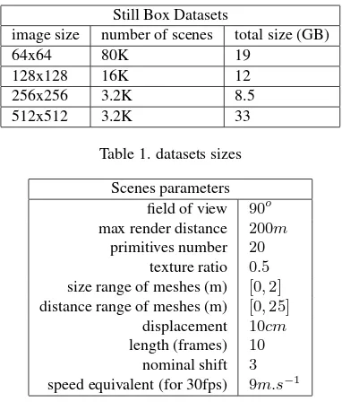
Still Box Datasets
image size number of scenes total size (GB)
64x64 80K 19
128x128 16K 12
256x256 3.2K 8.5
512x512 3.2K 33
Table 1. datasets sizes
Scenes parameters field of view 90o max render distance 200m
primitives number 20
texture ratio 0.5
size range of meshes (m) [0,2]
distance range of meshes (m) [0,25]
displacement 10cm
length (frames) 10
nominal shift 3
speed equivalent (for 30fps) 9m.s−1
Table 2. datasets parameters
movement. Some provide IMU data along with frames (Smith et al., 2009,Gaidon et al., 2016), that could be used to compensate rotation but their size in terms of different scenes would only let us use them for finetuning or validation.
3. STILL BOX DATASET
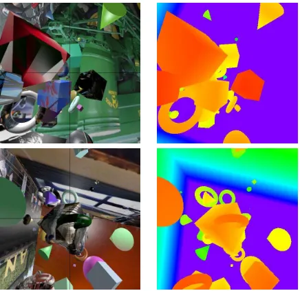
From our understanding of the lack of an adequate dataset for our problem, we decided to design our own synthetic dataset. We used the rendering softwareBlenderto generate an arbitrary number of random rigid scenes, composed of basic 3d primitives (cubes, spheres, cones and tores) randomly textured from an im-age set scrapped fromFlickr(see Fig 2).
These objects are randomly placed and sized in the scene, so that they are mostly in front of the camera, with possible variations including objects behind camera, or even camera inside an object. Scenes in which camera goes through objects are discarded. To add difficulty we also applied uniform textures on a proportion of the primitives. Each primitive thus has a uniform probability (corresponding to texture ratio) of being textured from a color ramp and not from a photograph.
Walls are added at large distances as if the camera was inside a box (hence the name). The camera is moving at a fixed speed value, to a uniformly distributed random direction, which remains constant for each sequence. It can be anything from forward/back-ward movement to lateral movement (which is then equivalent to stereo vision). Tables 1 and 2 show a summary of our scenes parameters. They can be changed at will, and are stored in a metadata JSON file to keep track of it. Our dataset is then com-posed of 4 sub-datasets with different resolutions, 64px dataset being the largest in terms of number of samples, 512px being the heaviest in data.
4. END-TO-END LEARNING OF DEPTH INFERENCE 4.1 Why not disparity ?
Figure 2. Some examples of our renderings with associated depth maps (red is close, violet is far)
very convincing methods (Ilg et al., 2016,Kendall et al., 2017). Knowing depth and displacement in our dataset, one could think it is easy to get disparity, train a network for it using existing op-tical flow methods, and get the depth map indirectly. The link between disparity and depth is actually prone to large errors. To understand why, we can consider a picture with(u, v)
coordi-nates, and optical center atP0 =
u0
v0
, and define our system
as follows:
Definition 1 Disparityδ(P)is defined here by the norm of the velocity flow,flow(P)=
Definition 2 Focus of Expansion is defined by the pointΦwhere each flow vectorflow(P)=
from. Note that this property is only true in a rigid scene and without rotation. One can note that for a pure translation,Φis the projection of the displacement vector of the camera onto its own focal plane.
Theorem 1 For a random rotation-less displacement of normV
of a pinhole camera, with a focal lengthf, depthζ(P)is an ex-plicit function of disparityδ(P), focus of expansionΦand optical centerP0
This result (proved in annex A) is in a useful form for limit values. Lateral movement corresponds to||−−→P0Φ|| →+∞and then
lim
||−P−0→Φ||→+∞
ζ(P) = f V
δ(P)
When approachingΦ, knowing that depth is a bounded positive value, we can deduce:
δ(P) ∝
Limit of disparity in this case is0and we use its inverse. As a consequence, small errors on disparity estimation will result in diverging values of depth near the focus of expansion, while it corresponds to the direction the camera is moving to, which is clearly problematic for depth-based obstacle avoidance.
Given the random direction of our camera’s displacement, com-puting depth from disparity is therefore much harder than for a classic stereo rig. To tackle this problem, we decided to set up an end-to-end learning workflow, by training a neural network to explicitly predict the depth of every pixel in the scene, from an image pair with constant displacement valueD0.
4.2 Dataset augmentation
The way we store data in 10 images long videos, with each frame paired with its ground truth depth, allows us to set a posteri-oridistances distribution with a variable temporal shift between two frames. For example, using a baseline shift of 3 frames, we can assume a depth three times greater than for two consecutive frames (shift of 1). A shift of 0 will result in an infinite depth, capped to a certain value (here 100m). In addition, we can also consider negative shift, which will only change displacement di-rection without changing speed value. These augmentation tech-niques allow us, given a fixed dataset size, to get more evenly distributed depth values to learn, and also to decorrelate appear-ance from depth, preventing any over-fitting during training, that would result in a scene recognition algorithm and would perform poorly on a validation set.
4.3 Depth Inference training
Our network is broadly inspired from FlowNetS (Dosovitskiy et al., 2015) (initially used for flow inference) and called Depth-Net. It is described Fig 3. Every convolution (apart from depth module) is followed by a Spatial Batch Normalization and ReLU activation layer. Batch normalization helps convergence and sta-bility during training by normalizing a convolution’s output over a batch of multiple inputs (Ioffe and Szegedy, 2015), and Recti-fied Linear Unit (ReLU) is the typical activation layer (Xu et al., 2015). One should note that FlowNetS initially used LeakyReLU which has a non-null slope for negative values, but tests showed that ReLU performed better for our problem. The main idea be-hind this network is that upsampled feature maps are concate-nated with corresponding earlier convolution outputs. Higher semantic information is then associated with information more closely linked to pixels (since it went through less strided con-volutions) which is then used for reconstruction. It is also im-portant to note that contrary to FLowNetS, our network does not need to be completely agnostic to optical flow structure, as it will be given frame pairs from rigid scenes, which dramatically low-ers our problem’s dimensionality. We therefore assumed that a thinner network would perform as well as a simple variation of FlowNetS and used half the feature maps for each layer.
Typical Conv Module SpatialConv, 3x3 SpatialBatchNorm ReLU
Typical Deconv Module SpatialConvTranspose, 4x4 SpatialConv, 3x3
SpatialBatchNorm ReLU
Input image pair
Conv1, stride 2
Conv2, stride 2
Conv3, stride 2
Conv3.1
Conv4, stride 2
Conv4.1
Conv5, stride 2
Conv5.1
Conv6, stride 2
Conv6.1
Deconv5
Concat5
Deconv4
Concat4
Deconv3
Concat3
Deconv2
Concat2
Depth2
Final depth output MultiScale
L1 Loss Depth6
Up Depth6
Depth5
Up Depth5
Depth4
Up Depth4
Depth3
Up Depth3 6xHxW
32x1/2Hx1/2W
64x1/4Hx1/4W
128x1/8Hx1/8W
256x1/16Hx1/16W
256x1/32Hx1/32W
512x1/64Hx1/64W
256x1/32Hx1/32W
128x1/16Hx1/16W
64x1/8Hx1/8W
32x1/4Hx1/4W
1x1/64Hx1/64W
1x1/32Hx1/32W
1x1/16Hx1/16W
1x1/8Hx1/8W
1x1/4Hx1/4W
Figure 3. DepthNet structure parameters, Conv and Deconv modules detailed above
Figure 4. result for 64x64 images, upper-left: input (before being downscaled to 64x64), lower-left: Ground Truth depth,
lower-right: our network output (16x16), upper-right: error (green is no error, red is over-estimated depth, blue is
under-estimated)
and disparity, such as FlowNetC or GC-Net (Kendall et al., 2017) among many others. The main point of this experimentation is to show that direct depth estimation can be beneficial regarding unknown translation. Like FlowNetS, we use a multi-scale crite-rion, with a L1 reconstruction error for each scale.
Loss= X
s∈scales
γs
1
HsWs X
i X
j
|outputs(i, j)−ζs(i, j)|
(1) where
• γs is the weight of the scale, arbitrarily set toWs in our experiments.
• (Hs, Ws) = (1/2nH,1/2nW)are the height and width of the output.
• ζsis the scaled depth groundtruth, using average pooling.
As said earlier, we apply data augmentation to the dataset using different shifts, along with classic methods such as flips and rota-tions.
Fig 4 shows results from 64px dataset. Like FlowNetS, results are downsampled by a factor of 4, which gives 16x16 Depth Maps.
One can notice that although the network is still fully convolu-tional, feature map sizes go down to 1x1 and then behave exactly like a Fully Connected Layer, which can serve to implicitly figure out motion direction, and spread this information across the out-puts. The second noticeable fact is that near FOE, (see Fig 5 for pixel-wise depth error according to distance from FOE) the net-work has no difficulty in inferring depth, which means that it uses neighbor disparity and interpolates when no other information is available.
Figure 5. mean depth error as a function of distance from FOE, for DepthNet64
Network L1Error RMSE
train test train test FlowNetS64 1.69 4.16 4.25 7.97 DepthNet64 2.26 4.49 5.55 8.44 FlowNetS64→128→256→512 0.658 2.44 1.99 4.77 DepthNet64→128 1.20 3.07 3.43 6.30 DepthNet64→128→256 0.876 2.44 2.69 4.99 DepthNet64→128→256→512 1.09 2.48 2.86 4.90 DepthNet64→512 1.02 2.57 2.81 5.13 DepthNet512 1.74 4.59 4.91 8.62
Table 3. quantitative results for depth inference networks. FlowNetS is modified with 1 channel outputs (instead of 2 for
inferring flow), and trained from scratch for depth with Still Box. Subscript indicates fine tuning process.
4.4 From 64px to 512px Depth inference
One could think that a fully convolutional network such as ours can not solve depth extraction for pictures greater than 64x64. The main idea is that for a fully convolutional network, each pixel is applied the same operation. For disparity, this makes sense be-cause the problem is essentially similarity from different picture shifts. Wherever we are on the picture, the operation is the same. For depth inference when FOE is not diverging (forward move-ment is non negligible), Theorem 1 shows that once you know the FOE, distinct operations should be done depending on the distance from the FOE and from the optical centerP0. The only possible strategy for a fully convolutional network would be to also compute the position in the image and to apply the compen-sating scaling to the output.
This problem then seems very difficult, if not impossible for a network as simple as ours, and if we run the training directly on
Network size 980Ti
Quadro
K2200m TX1
1 8 1 8 1 8
FlowNetS64 39.4 225 153 76 41 29 14
DepthNet64 7.33 364 245 190 124 70 40
FlowNetS512 39.4 69 8.8 16 N/A 2.8 N/A
DepthNet128 7.33 294 118 171 75 51 15
DepthNet256 7.33 178 36 121 30 39 3.2 DepthNet512 7.33 68 8.8 51 7.6 9.2 N/A Table 4. Size (millions of parameters) and Inference speeds (fps)
on different devices. Batch sizes are1and8(when applicable). A batch size of8means8depth maps computed at the same time
Figure 7. some results on real images input. Up is from a Bebop drone footage, down is from a gimbal stabilized smartphone
video
512x512 images, the network fails to converge to better results than with 64x64 images (while better resolution would help get-ting more precision). However, if we take the converged network and apply a fine-tuning on it with 512x512 images, we get much better results. Fig 6 shows training results for mean L1 recon-struction error, and shows that our deemed-impossible problem seems to be easily solved with multi-scale fine-tuning. As Ta-ble 3 shows, best results are obtained with multiple fine-tuning, with intermediate scales 64, 128, 256, and finally 512pixels. FlowNetS is performing better than DepthNet but by a fairly light margin while being 5 times heavier and most of the time much slower, as shown in Table 4. As our network is leveraging the re-duced dimensionality of our dataset due to its lack of rotation, it is hard to compare our method to anything else apart from this vari-ation of FlowNetS. Disparity estimvari-ation is equivalent to a lateral translation, on which our network has also been trained, and then could be used to compare to other algorithms but this reduced context seems unfair compared to methods specifically designed for it and we decided not to include it.
Fig 6 and 7 shows qualitative results from our validation set, and from real condition drone footage, on which we were careful to avoid camera rotation. These results did not benefit from any fine-tuning from real footage, indicating that our Still Box Dataset, al-though not realistic in its scenes structures and rendering, appears to be sufficient for learning to produce decent depth maps in real conditions.
5. UAV NAVIGATION USE-CASE
We trained a network for depth inference from a moving camera, assuming its velocity is always the same. When running during flight, such a system can easily deduce the real depth map from the drone displacementDtbetween the two frames, knowing that the training displacement wasD0(here0.3m)
ζ(t) = Dt
D0
DepthN et(It, It−1) (2)
One of the drawbacks of this learning method is that thefvalue (which is focal length divided by pixel size) of our camera must be the same as the one used in training. Our dataset creation framework however allows us to change this value very easily for training. One must also be sure to have pinhole equivalent frames like during training.
Depending of the depth distribution of the groundtruth depth map, it may be useful to adjust frame shift. For example, when flying high above the ground, big structure detection and avoidance re-quires knowing precise distance values that are outside the typical range of any RGB-D sensor. The logical strategy would then be to increase the temporal shift between the frame pairs provided to DepthNet as inputs.
More generally, one must ensure a well distributed depth map from 0 to 100m to get high quality depth inference. This prob-lem can be solved by deducing optimal shift∆tfrom precedent inference distribution, e.g:
∆t+1= ∆t
Eζ
E0
whereE0is an arbitrarily chosen value around which our network has the best accuracy, e.g. 50m, because our network outputs from 0 to 100m, andEζis the mean of precedent output, i.e.:
Eζ=
1
HW
X
i,j
DepthN et(It, It−∆t)i,j
6. CONCLUSION AND FUTURE WORK We proposed a novel way of computing dense depth maps from motion, along with a very comprehensive dataset for stabilized footage analysis. This algorithm can be used for depth-based sense and avoid algorithm in a very flexible way, in order to cover all kinds of path planning, from collision avoidance to long range obstacle bypassing.
Future works include using batch inference to compute depth with multiple shifts∆t,i. As shown in Table 4, batch size greater than 1 can be used to some extent (especially for low resolution) to efficiently compute multiple depth maps.
ζi(t) =DepthN et(It, It−∆i,t)
These multiple depth maps can then be either combined to con-struct a high quality depth map, or used separately to run two dif-ferent obstacle avoidance algorithm, e.g. one dedicated for long range path planning (and then a high value∆i,t) and the other for reactive and short range collision avoidance (with low∆i,t). While one depth map will display closer areas at zero distance but further regions with precision, the other will set far regions to infinity (or 100m for DepthNet) but closer region with high resolution.
We also consider an implementation of a real dataset for fine tun-ing, using UAVs footages and either a preliminary thorough 3D offline scan or groundtruth-less techniques (Zhou et al., 2017). This would allow us to measure quantitative quality of our net-work for real footages and not only subjective as for now.
REFERENCES
Cadena, C., Carlone, L., Carrillo, H., Latif, Y., Scaramuzza, D., Neira, J., Reid, I. and Leonard, J. J., 2016. Past, present, and future of simultaneous localization and mapping: Toward the robust-perception age. IEEE Transactions on Robotics32(6), pp. 1309–1332.
Coombs, D., Herman, M., Hong, T.-H. and Nashman, M., 1998. Real-time obstacle avoidance using central flow divergence, and peripheral flow.IEEE Transactions on Robotics and Automation
14(1), pp. 49–59.
De N´o, R, L., 1933. Vestibulo-ocular reflex arc. Archives of Neurology & Psychiatry30(2), pp. 245–291.
Dosovitskiy, A., Fischer, P., Ilg, E., H¨ausser, P., Hazrba, C., Golkov, V., v.d. Smagt, P., Cremers, D. and Brox, T., 2015. Flownet: Learning optical flow with convolutional networks. In:
IEEE International Conference on Computer Vision (ICCV).
Eigen, D., Puhrsch, C. and Fergus, R., 2014. Depth map predic-tion from a single image using a multi-scale deep network. In:
Advances in neural information processing systems, pp. 2366– 2374.
Firman, M., 2016. RGBD Datasets: Past, Present and Future. In:CVPR Workshop on Large Scale 3D Data: Acquisition, Mod-elling and Analysis.
Gaidon, A., Wang, Q., Cabon, Y. and Vig, E., 2016. Virtual worlds as proxy for multi-object tracking analysis. In: Proceed-ings of the IEEE Conference on Computer Vision and Pattern Recognition, pp. 4340–4349.
Garg, R., G, V. K. B. and Reid, I. D., 2016. Unsupervised CNN for single view depth estimation: Geometry to the rescue.CoRR.
Geiger, A., Lenz, P. and Urtasun, R., 2012. Are we ready for autonomous driving? the kitti vision benchmark suite. In: Com-puter Vision and Pattern Recognition (CVPR), 2012 IEEE Con-ference on, IEEE, pp. 3354–3361.
Giusti, A., Guzzi, J., Cires¸an, D. C., He, F.-L., Rodr´ıguez, J. P., Fontana, F., Faessler, M., Forster, C., Schmidhuber, J., Di Caro, G. et al., 2016. A machine learning approach to visual perception of forest trails for mobile robots.IEEE Robotics and Automation Letters1(2), pp. 661–667.
Godard, C., Mac Aodha, O. and Brostow, G. J., 2017. Unsuper-vised monocular depth estimation with left-right consistency. In:
CVPR.
Hadsell, R., Sermanet, P., Ben, J., Erkan, A., Scoffier, M., Kavukcuoglu, K., Muller, U. and LeCun, Y., 2009. Learning long-range vision for autonomous off-road driving. Journal of Field Robotics26(2), pp. 120–144.
Hitomi, E. E., Silva, J. V. and Ruppert, G. C., 2015. 3d scan-ning using rgbd imaging devices: A survey. In:Developments in Medical Image Processing and Computational Vision, Springer, pp. 379–395.
Ilg, E., Mayer, N., Saikia, T., Keuper, M., Dosovitskiy, A. and Brox, T., 2016. Flownet 2.0: Evolution of optical flow estimation with deep networks.arXiv preprint arXiv:1612.01925.
Ioffe, S. and Szegedy, C., 2015. Batch normalization: Acceler-ating deep network training by reducing internal covariate shift.
arXiv preprint arXiv:1502.03167.
Kendall, A., Martirosyan, H., Dasgupta, S., Henry, P., Kennedy, R., Bachrach, A. and Bry, A., 2017. End-to-End Learning of Ge-ometry and Context for Deep Stereo Regression.ArXiv e-prints.
Klein, G. and Murray, D., 2007. Parallel tracking and mapping for small ar workspaces. In:Mixed and Augmented Reality, 2007. ISMAR 2007. 6th IEEE and ACM International Symposium on, IEEE, pp. 225–234.
Krizhevsky, A., Sutskever, I. and Hinton, G. E., 2012. Imagenet classification with deep convolutional neural networks. In: Ad-vances in neural information processing systems, pp. 1097–1105.
LeCun, Y., Muller, U., Ben, J., Cosatto, E. and Flepp, B., 2005. Off-road obstacle avoidance through end-to-end learning. In:
NIPS, pp. 739–746.
Long, J., Shelhamer, E. and Darrell, T., 2015. Fully convolutional networks for semantic segmentation. In: The IEEE Conference on Computer Vision and Pattern Recognition (CVPR).
Luo, W., Schwing, A. G. and Urtasun, R., 2016. Efficient deep learning for stereo matching. In: Proceedings of the IEEE Con-ference on Computer Vision and Pattern Recognition, pp. 5695– 5703.
Menze, M. and Geiger, A., 2015. Object scene flow for au-tonomous vehicles. In:Proceedings of the IEEE Conference on Computer Vision and Pattern Recognition, pp. 3061–3070.
Michels, J., Saxena, A. and Ng, A. Y., 2005. High speed obsta-cle avoidance using monocular vision and reinforcement learn-ing. In: Proceedings of the 22nd international conference on Machine learning, ACM, pp. 593–600.
Mur-Artal, R. and Tardos, J. D., 2016. Orb-slam2: an open-source slam system for monocular, stereo and rgb-d cameras.
arXiv preprint arXiv:1610.06475.
N.Mayer, E.Ilg, P.H¨ausser, P.Fischer, D.Cremers, A.Dosovitskiy and T.Brox, 2016. A large dataset to train convolutional networks for disparity, optical flow, and scene flow estimation. In: IEEE International Conference on Computer Vision and Pattern Recog-nition (CVPR). arXiv:1512.02134.
Pizzoli, M., Forster, C. and Scaramuzza, D., 2014. REMODE: Probabilistic, monocular dense reconstruction in real time. In:
IEEE International Conference on Robotics and Automation (ICRA).
Saxena, A., Chung, S. H. and Ng, A. Y., 2005. Learning depth from single monocular images. In:NIPS, Vol. 18, pp. 1–8.
Scharstein, D. and Szeliski, R., 2002. A taxonomy and evaluation of dense two-frame stereo correspondence algorithms. Interna-tional journal of computer vision47(1-3), pp. 7–42.
Smith, M., Baldwin, I., Churchill, W., Paul, R. and Newman, P., 2009. The new college vision and laser data set.The International Journal of Robotics Research28(5), pp. 595–599.
Sturm, J., Engelhard, N., Endres, F., Burgard, W. and Cremers, D., 2012. A benchmark for the evaluation of rgb-d slam systems. In: Proc. of the International Conference on Intelligent Robot Systems (IROS).
Weinzaepfel, P., Revaud, J., Harchaoui, Z. and Schmid, C., 2013. DeepFlow: Large displacement optical flow with deep matching. In: ICCV 2013 - IEEE International Conference on Computer Vision, IEEE, Sydney, Australia, pp. 1385–1392.
Xu, B., Wang, N., Chen, T. and Li, M., 2015. Empirical evalua-tion of rectified activaevalua-tions in convoluevalua-tional network.CoRR.
Zbontar, J. and LeCun, Y., 2015. Computing the stereo matching cost with a convolutional neural network. In:Proceedings of the IEEE Conference on Computer Vision and Pattern Recognition, pp. 1592–1599.
Zhou, T., Brown, M., Snavely, N. and Lowe, D. G., 2017. Unsu-pervised learning of depth and ego-motion from video. In:CVPR.
Zingg, S., Scaramuzza, D., Weiss, S. and Siegwart, R., 2010. Mav navigation through indoor corridors using optical flow. In:
Robotics and Automation (ICRA), 2010 IEEE International Con-ference on, IEEE, pp. 3361–3368.
A. APPENDIX A : PROOF OF THEOREM 1 For a random rotation-less displacement of normV, depthζ(P)
is an explicit function of disparityδ(P), focus of expansionΦand optical centerP0
PROOF We assume no rotation. which meansΦis projection of B on A.
relative movement ofPXY Zis−m
so we have
Similarly, withv, we get:
du= mz
Z+mz (uB−Φu)
dv= mz
Z+mz(vB−Φv)
(4)
We consider disparityδ(P)norm of the flow
du dv
expressed in
frame B (which is correlated to depth at this frame).
∀P=
Consequently, we can deduce depth at frame B from disparity :
∀P=
From our dataset construction, we know thatm2