Intraseasonal variations of surface and subsurface currents off Java as
simulated in a high-resolution ocean general circulation model
Iskhaq Iskandar,1,2 Tomoki Tozuka,1Hideharu Sasaki,3Yukio Masumoto,1,4 and Toshio Yamagata1,4
Received 11 January 2006; revised 9 August 2006; accepted 25 August 2006; published 21 December 2006.
[1] A high-resolution ocean general circulation model (OGCM) is used to explore dynamics of intraseasonal variability in surface and subsurface currents off Java. The results indicate that the surface current, the so-called South Java Coastal Current (SJCC), is dominated by variations with a period of 90 days. In the subsurface current, which is referred to as the South Java Coastal Undercurrent (SJCU), 60-day variations are the most prominent feature. A normal mode analysis demonstrates that the first baroclinic mode is the leading mode, which accounts for 70% of the total variance, whereas the second baroclinic mode explains 24% of the total variance. The 90-day variations in the SJCC captured mostly by the first baroclinic mode are found to be primarily driven by winds. Those are associated with propagation of the first baroclinic Kelvin waves generated in the central equatorial Indian Ocean. On the other hand, the 60-day variations in the SJCU enhanced by wind forcing over the eastern equatorial Indian Ocean off Sumatra are mostly captured by the second baroclinic mode.
Citation: Iskandar, I., T. Tozuka, H. Sasaki, Y. Masumoto, and T. Yamagata (2006), Intraseasonal variations of surface and subsurface currents off Java as simulated in a high-resolution ocean general circulation model,J. Geophys. Res.,111, C12015, doi:10.1029/2006JC003486.
1. Introduction
[2] The surface current off Java, so-called the South Java Coastal Current (SJCC), is considered to be driven by the monsoonal winds over the Indian Ocean and the Indonesia archipelago. It actually undergoes a dramatic seasonal var-iation. During the northwest monsoon season (December – April), it flows southeastward along the coast and reaches the maximum strength in February. In contrast, the prevailing southeasterly winds reverse the direction of the SJCC from June to October, and the flow reaches its peak in August [Wyrtki, 1961;Quadfasel and Cresswell, 1992].
[3] To understand its higher-frequency variability,
Sprintall et al. [1999], on the basis of in situ measurement of currents, temperature and salinity off Java from March 1997 to March 1998, discussed the modulation of the SJCC on a semiannual timescale and clarified the important of the remote wind forcing over the equatorial Indian Ocean during the monsoon breaks (April/May and October/ November) in generating eastward-propagating equatorial Kelvin waves.Qiu et al.[1999], using a 11=2-layer reduced-gravity model, demonstrated that the maximum eastward transport associated with the SJCC occurs during the
transition seasons of monsoon. More recently, Qu and Meyers [2005a] have found that the annual variation is dominant in the upper part of SJCC, and that the semiannual variation is dominant in the deeper part.
[4] The intraseasonal fluctuations have also been observed in the sea level variation along the southern coast of Sumatra and Java [Arief and Murray, 1996; Iskandar et al., 2005], in the outflow straits of the Indonesian Throughflow (ITF) [Chong et al., 2000; Potemra et al., 2002], and in the South Equatorial Current (SEC) [Feng and Wijffels, 2002]. However, the intraseasonal fluctuations in the SJCC have been of less concern because those are not very well resolved in observational data. In this regard, analysis on the hydrographic records of the Indo-Australian basin provided descriptions of the subsurface flow along the coastal waveguide off Java. Near the southern coast of Bali, two hydrographic sections investigated in August 1989 and February 1992 show a mean eastward flow in the depth of about 300 – 800 m [Fieux et al., 1994, 1996]. This eastward flow is characterized by high salinity and low oxygen concentration of the Northern Indian Ocean Water [Fieux et al., 1994, 1996; Wijffels et al., 2002]. Unlike the SJCC that recirculates into the Indian Ocean by feeding into the SEC upon reaching the Lombok Strait, this eastward flow in the deeper layer penetrates farther east [Sprintall et al., 2002; Wijffels et al., 2002]. Unfortunately, however, the analysis is only based on one-time cruises. Therefore the long-term variations cannot be captured. Moreover, the large seasonal to interannual variations that are prominent in this region can alias the measurement if the observation periods are not long enough.
JOURNAL OF GEOPHYSICAL RESEARCH, VOL. 111, C12015, doi:10.1029/2006JC003486, 2006 Click
Here for
Full Article
1Department of Earth and Planetary Science, Graduate School of
Science, University of Tokyo, Tokyo, Japan.
2
On leave from University of Sriwijaya, South Sumatra, Indonesia
3Earth Simulator Center, JAMSTEC, Yokohama, Kanagawa, Japan. 4
Also at Frontier Research Center for Global Changes, JAMSTEC, Yokohama, Kanagawa, Japan.
[5] This study therefore aims to provide a comprehensive description of the SJCC and the current system underneath the SJCC with a special emphasis on the intraseasonal variability using results from a high-resolution OGCM. The present study will address following questions. First, what is the dominant period of variability in the surface and subsurface currents off Java? What driving mechanism is responsible for the variations? How are these current variations related to propagation of remotely forced Kelvin waves? The rest of the paper is organized as follows. A concise explanation of the model used in this study and its validation are given in the next section. Characteristics of the zonal currents off Java are described in section 3. In section 4, we apply a normal mode analysis to the model zonal current off Java to show dominance of the intra-seasonal variability. Driving mechanisms for the intrasea-sonal variability are discussed in section 5, and the final section is reserved for summary.
2. Ocean Model 2.1. Model Description
[6] The model used in this study is a high-resolution OGCM developed for the Earth Simulator (hereafter referred to as OFES). For detailed description of the model, readers are referred to Masumoto et al. [2004] and refer-ences therein. The model is based on the Modular Ocean Model (MOM3) and covers a near-global region extending from 75°S to 75°N. The horizontal resolution is 1/10°and there are 54 levels in the vertical with variable grid width. There are 34 vertical levels in the upper 1000 m, which seem to be sufficient to resolve current variability in the upper ocean. The model has realistic topography derived from the 1/30° OCCAM bathymetry data set. At the northern and southern artificial boundaries, temperature and salinity fields are relaxed to the monthly mean clima-tology of World Ocean Atlas 1998. A biharmonic smoother is applied for the horizontal mixing, whereas the vertical mixing is based on the KPP boundary layer mixing scheme. The surface heat and fresh water flux were specified using bulk formula with atmospheric data set obtained from monthly mean climatology of NCEP/NCAR reanalysis data.
Also, the surface salinity is relaxed to monthly mean climatology of the WOA98 with a timescale of 6 days.
[7] The model, which is initially at rest, is first spun up for 50 years with initial temperature and salinity fields that are derived from the annual mean of WOA98. It is then integrated for 54 years from January 1950 through December 2003 using the daily mean NCEP/NCAR reanalysis data.
2.2. Model Validation
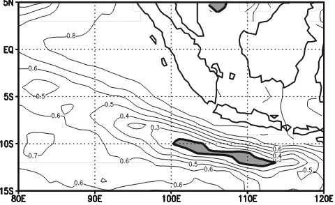
[8] To verify the model results prior to the analysis, we have first analyzed the variability in sea surface height anomaly (SSHA). The model SSHA corresponds remark-ably well to the satellite altimetry data of TOPEX/Poseidon, in particular, near the southern coast of Sumatra and Java; the correlation coefficient is larger than 0.7 (Figure 1). Farther south, however, the correlation coefficients drop below the confidence level. We suggest that this is due to high eddy activities, which are not well simulated in our model.
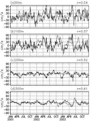
[9] Then, we have compared the hindcast zonal currents with the observed zonal current from the moored ADCP at 90°E right on the equator [Masumoto et al., 2005]. Four examples at depths of 50 m, 100 m, 200 m and 300 m are shown in Figures 2a – 2d. We see that the model represents the observed variations relatively well at all depths as the correlation coefficients are larger than 0.5.
[10] Given that the OFES has a relatively good skill in simulating observed variability, we expect that the model can provide some insight into the zonal current variability off Java. The simulation results for the period of 1990 – 2003 are used for this purpose.
3. Characteristics of the Surface and Subsurface Currents off Java
3.1. General Characteristics of the Mean Flow
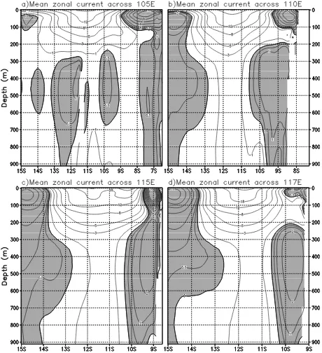
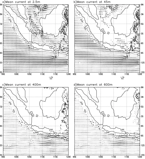
[11] Vertical sections of climatological mean zonal cur-rents across selected longitudes are shown in Figures 3a – 3d. There are two distinct eastward flows in the upper layer and a broader westward flow. One eastward flow is confined to the coast of Java, while the other is located south of 14°S and extends farther south to the coast of Australia (not shown). The former corresponds to the SJCC. The westward flow is centered at 12°S and is associated with the SEC as previously suggested [Feng and Wijffels, 2002]. Although there are some unresolved issues related to the generation mechanism of the SEC, we focus on the variability off Java. [12] We here describe general features of the surface and subsurface currents off Java based on these zonal current sections. The surface current corresponding to the SJCC is a relatively shallow flow with the maximum eastward velocity occurs at about 50 m. Flow exceeding 5 cm/s does not extend below 100 m at all sections. As previously suggested [Sprintall et al., 2002;Wijffels et al., 2002], the flow is regulated by the ITF through the Lombok Strait (Figure 3d) and recirculates into the Indian Ocean by feed-ing the SEC (Figures 4a and 4b).
[13] The core of the subsurface current exists approxi-mately at 400 m depth with peak velocity of about 3 cm/s (Figures 3c and 4c). We note that the amplitude of subsur-face flow increases eastward along the coast (Figures 3c, 3d, 4c, and 4d). This subsurface flow penetrates farther east and
partly enters the Savu Sea through the Sumba Strait, but a large part flows farther east along the western coast of Sumba Island and then joins the ITF from the Timor Sea (Figures 4c and 4d).
[14] In this study, we define the SJCC as the surface current above 150 m; the subsurface current below 150 m down to 1000 m is denoted as the South Java Coastal Undercurrent (SJCU).
3.2. Intraseasonal Variations
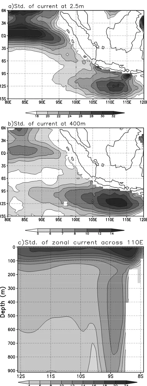
[15] Standard deviations of the 20 – 120 days band-pass filtered model surface velocity show that the highest vari-ability occurs in the equatorial Indian Ocean (Figure 5a). Here we have used the wavelet filter of Torrence and Compo [1998]. The present result is consistent with the previous observational study [Masumoto et al., 2005], which demonstrated that energetic intraseasonal variations in westerly winds drive the eastward jet along the equatorial Indian Ocean. In addition, the region off Java shows relatively large variations in both surface and subsurface layer (Figures 5a and 5b). In order to have a vertical
distribution of the intraseasonal variations off Java, we have calculated a standard deviation of 20 – 120 days band-pass filtered model zonal current across 110°E (Figure 5c). As expected, the maximum variation is evident above the depth of 100 m. In addition, there is also a core of relatively high variations from 200 to 800 m, suggesting strong subsurface variations underneath the SJCC. Those seem to be related to variations of the SJCU.
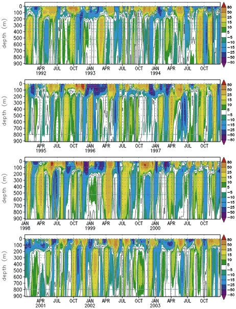
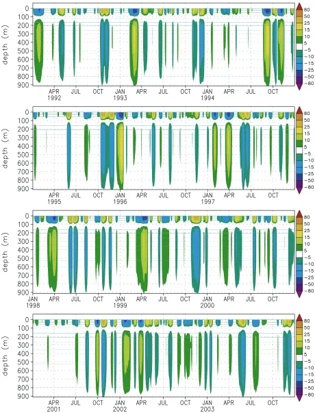
[16] The time evolution of zonal currents off Java is further analyzed using the time-depth section of the model zonal current at 8.6°S, 110°E between 3 January 1992 and 31 December 2003 (Figure 6). The most striking feature of the SJCC is the presence of alternating eastward and westward currents with a period less than a month. The stronger eastward current exceeding 40 cm/s mostly takes place during monsoon breaks (April/May and October/ November), which corresponds to the Yoshida-Wyrtki jets. However, there are also strong eastward currents during boreal summer (June – August). A recent numerical study [Senan et al., 2003] has shown that the atmospheric intra-seasonal oscillation during boreal summer could generate
Figure 2. Comparisons of the zonal currents between the model (dashed line) and the observation (solid line) at 90°E on the equator.
intraseasonal oceanic eastward jet in the eastern equatorial Indian Ocean. Thus we hypothesize that the intraseasonal variations in the SJCC during boreal summer may be related to the atmospheric intraseasonal variations over the equa-torial Indian Ocean. The subsurface SJCU, on the other hand, shows alternate eastward and westward currents at lower frequencies with significant energy at about two months period.
[17] To know the dominant period of variability in the SJCC and SJCU, spectra of the depth-averaged zonal currents off Java are calculated (Figure 7). Within the
intraseasonal timescale, the SJCC shows four significant peaks at about 25, 35, 50 and 90 days, among which the 90-day signal is dominant. The SJCU, on the other hand, shows dominant variability with a period of about 60 days. [18] At lower frequencies, both the SJCC and the SJCU show maximum variance at a semiannual period (182 days) and somewhat weaker variance at an annual period (365 days). The semiannual signal appears to be related to the incoming semiannual Kelvin waves (i.e., Yoshida-Wyrtki jets) generated in the equatorial Indian Ocean, while annually reversing monsoon winds over the Indonesian
Figure 4. Mean currents (cm/s) in the southeastern tropical Indian Ocean at (a) 2.5 m, (b) 45 m, (c) 400 m, and (d) 600 m.
region are a plausible forcing mechanism for the annual variation.
4. Intraseasonal Variations From a Normal Mode Analysis
[19] Following Gill and Clarke [1974], we solve the governing equations for wind-forced flow by adopting a modal decomposition method. The vertical eigenfunction,
yn(z), of mode numbernsatisfies d
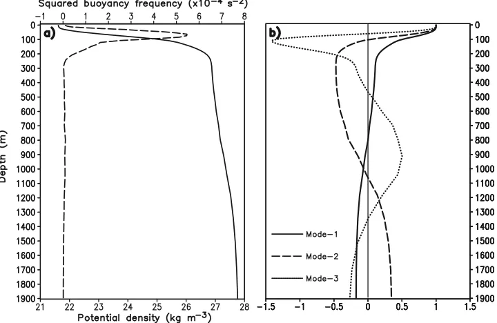
where Nbis the Bru¨nt-Va¨isa¨la¨ frequency associated with the background state, and cnis the phase speed for the moden. The eigenfunction,yn(z), is normalized so that yn(0) = 1. Figure 8a shows the density and the Bru¨nt-Va¨isa¨la¨ frequency profiles at 8.6°S, 110°E from which the vertical eigenfunctions were calculated. As seen in Figure 8b, the first vertical mode has a zero crossing around 800 m depth. The second vertical mode has two zero crossing points; one is at around 100 m depth, and another at about 1100 m depth. The third vertical mode is more confined in the surface, with the first zero crossing at around 50 m depth, the second one at around 500 m depth, and the third one is at about 1350 m depth.
[20] The horizontal velocity is expressed as
u;v
where the barotropic mode (n = 0) is neglected in our calculations; the barotropic response is negligible with respect to the baroclinic response.
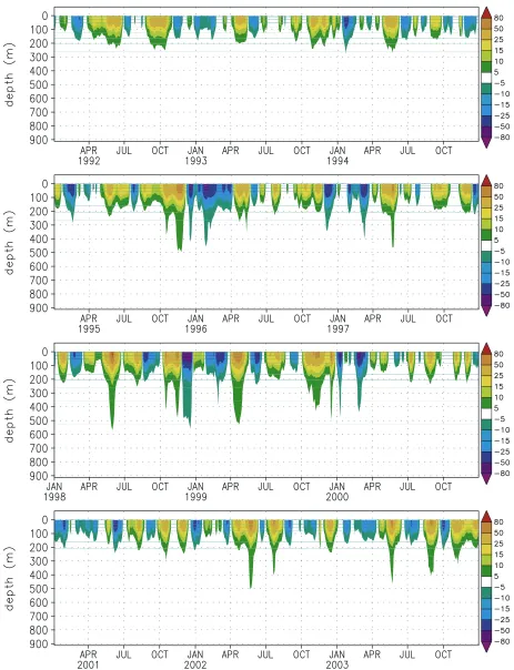
[21] Contributions from each vertical mode on the zonal current at 8.6°S, 110°E are calculated using equation (3) (Figures 9 – 11). The first mode, which accounts for 70% of the total variance, dominates the variability, while the second mode explains 24% of the total variance. In consis-tence with the present results,Sprintall et al.[2000] found that sea level variations along the southern coast of Indo-nesia are mostly dominated by the first vertical mode, which explains 76% of the total variance. Interestingly, the first mode mostly captures the variability of the SJCC (Figure 9), whereas the variability of the SJCU is mostly depicted by the second mode (Figure 10). Table 1 indicates quantita-tively the fractions of the variance for the first two modes at each depth. The first mode is more dominant in the upper layer (above150 m), while the second mode has signif-icant contributions in the lower layer between about 200 – 800 m. Below 1000 m, the first mode again dominates the variations.
[22] In order to evaluate the dominant frequency for each vertical mode, we have prepared Figure 12, which displays power spectra of the first two vertical modes. It is shown that the first mode has five significant peaks within the intraseasonal timescale: 25, 35, 50, 60 and 90 days, which
Figure 6. Time depth section of the model zonal currents (cm/s) at 8.6°S, 110°E for the period of 3 January 1992 to 31 December 2003. Zero contours are indicated with solid lines.
correspond to those of the SJCC (Figure 7). For the second mode, the most prominent intraseasonal peak is the 60-day signal corresponding to that of the SJCU.
5. Mechanism for Generating the Intraseasonal Variations
[23] The southeastern tropical Indian Ocean off Java is a region of a complex interplay between remote forcing from both the equatorial Indian and Pacific Ocean, and local
forcing associated with monsoonal winds over this region [Clarke and Liu, 1993;Qiu et al., 1999;Chong et al., 2000;
Sprintall et al., 2000; Potemra et al., 2002; Wijffels and Meyers, 2004; Iskandar et al., 2005]. Although an intrigu-ing basin-wide resonance was suggested as an additional forcing mechanism for the intraseasonal variations in the equatorial Indian Ocean [Cane and Moore, 1981; Han, 2005;Fu, 2006], we here focus only on direct wind forcing. Dominant parts of the intraseasonal variations, 90-day variations in the SJCC and 60-day variations in the SJCU, are examined here. A band-pass filter for the period of 75 – 105 days is applied to capture the 90-day signal, while the 60-day signal is selected by 54 – 69 days band-pass filter.
[24] The efficiency of the wind stress in exciting the vertical modes is analyzed by calculating the wind-stress coupling coefficient (Bn) for each mode [Moore
and Philander, 1978; McCreary, 1981]. First, the projec-tion of wind forcing onto each vertical mode is defined as
X;Y
ð Þ ¼ t
x;ty
ð Þ
Bn roðbcnÞ 1 2c
n
; ð4Þ
where tx, ty are the horizontal components of the wind stress vector, andr0is the mean water density. The coupling coefficient, which determines how each mode is related to the driving wind, is defined as
Bn¼ Hmix
Z 0
H
y2nð Þz dz
Z 0
Hmix ynð Þzdz
; ð5Þ
where Hmix is the mixed-layer depth. We define the depth of the mixed layer by specifying a density difference of 0.125 kg/m3 from the surface value. The coupling coefficients at different places are listed in Table 2. Not
Figure 7. Power spectra of the depth-averaged zonal currents for the upper layer (thin line) and the lower layer (thick line) at 8.6°S, 110°E.
Figure 9. Model zonal currents at 8.6°S, 110°E reconstructed from the first baroclinic mode.
Figure 11. As in Figure 9 but for sum of the first two baroclinic modes. Zero contours are indicated with solid lines.
surprisingly, only the first two modes are significantly excited, in agreement with results shown in Figures 9 – 11. In terms of the coupling coefficient, the first mode is excited more favorably in the eastern Indian Ocean, while the second mode is excited more favorably in the central and western Indian Ocean. The above important results have not been reported so far in the literature. The wind-stress coupling coefficient varies from location to location owing to difference in the basic stratification. T. Doi et al. (The wind-coupling coefficient in the global equatorial ocean, submitted to Journal of Physical Oceanography, 2005) have recently demonstrated that temporal as well as spatial variations of the thermocline depth lead to variations in the wind-stress coupling coefficient in the tropical oceans. In the eastern equatorial Indian Ocean, where the thermocline is thicker and less sharp, the first mode is more strongly excited, while the second mode is more efficiently excited in thinner and sharper thermocline regions of the central and western equatorial Indian Ocean.
5.1. The 90-Day Signal in the SJCC
[25] Figure 13a shows the lag correlation between the upper layer zonal currents at 8.6°S, 110°E and the wind stress along the equator, off Sumatra and off Java. It demonstrates that the currents at depth of 150 m, which are mostly explained by the first baroclinic mode, are forced
by the zonal wind stress distributed from the central to eastern equatorial Indian Ocean. The estimated phase speed is 259 ± 14 cm/s, which is close to that of the first baroclinic Kelvin waves shown in Table 2 and the observed estimate (276 cm/s) derived from the mean density profiles of the World Ocean Atlas 2001. This result is also remarkably in agreement with the correlation figure between the time series of the first vertical mode and the zonal wind stress, supporting the forcing region for the 90-day signal is located from the central to eastern equatorial Indian Ocean (Figure 13b).
[26] Contributions from the local forcing to the 90-day variations in the SJCC, however, are not negligible. The upper layer zonal currents at 8.6°S, 110°E also indicate significant correlation with the alongshore wind stress off Sumatra (Figure 13a). This is in agreement with previous observational [Sprintall et al., 1999;Chong et al., 2000] and numerical [Qiu et al., 1999] studies, which showed that the local wind forcing off Sumatra-Java enhances the intra-seasonal variations in this region. We note here that the time series of the first baroclinic mode also correlates with the alongshore wind stress off Sumatra (Figure 13b). This is consistent with the estimated wind-coupling coefficient shown in Table 2, where the first mode is more efficiently excited off Sumatra and Java.
[27] Since the remote equatorial winds and local winds are important in generating the intraseasonal variations of the SJCC, we have analyzed the spectral characteristic of the zonal wind stress along the equatorial Indian Ocean, the alongshore wind off Sumatra and the zonal winds off Java (Figures 14a – 14c). While the remote equatorial winds show a distinct spectral peak near 90-day over the wide zonal area in the central equatorial Indian Ocean, the local winds only exhibits weak energy in this period. This indicates that the 90-day variations in the SJCC are primarily related to winds
Table 1. Fractions of the Variance in the Model Zonal Current Explained by the First Two Vertical Modes at Each Deptha
2.5 m 54 m 108 m 148 m 288 m 319 m 526 m 605 m 796 m 1041 m 1184 m n=1 70.0 75.4 82.1 66.3 46.3 45.8 40.7 37.9 24.3 56.6 61.3 n=2 24.1 21.9 1.9 18.8 47.9 48.5 52.7 53.8 58.9 9.75 5.1
aFraction given as percent.
Figure 12. Power spectra of the time series shown in Figures 9 and 10 for the first baroclinic mode (thin line) and the second baroclinic mode (thick line).
Table 2. Characteristics of the First Two Vertical Modes at Different Locations
Location
Kelvin Wave Speed cn,
cm/s
Coupling Coefficient Bn,
Figure 13. (a) Time-longitude lag correlation between the upper layer zonal currents at 8.6°S, 110°E and the zonal wind stress along the equatorial Indian Ocean, alongshore wind stress off Sumatra, and zonal wind stress off Java, respectively. (b) A similar correlation between the time series of the first baroclinic mode from 8.6°S, 110°E and the same wind stress data. Eastward wind stress is associated with eastward currents. The 75 – 105 days band-pass filter has been applied to each data. Only correlation coefficients above 95% confidence level are plotted.
Figure 14. Variance-preserving spectra (dyn2cm4) of (a) the zonal wind stress along the equatorial Indian Ocean, (b) the alongshore winds off Sumatra, and (c) the zonal wind stress off Java.
along the equatorial Indian Ocean on this timescale even though they modulated by local winds.
5.2. The 60-Day Signal in the SJCU
[28] Response of the SJCU to direct wind forcing is examined by correlating the time series of the subsurface zonal current averaged between 150 and 1000 m with the zonal wind stress. Figure 15a demonstrates that the SJCU is significantly correlated with the zonal wind stress more confined in the eastern equatorial Indian Ocean off Sumatra, where intraseasonal atmospheric variability associated with the Madden-Julian Oscillation is very high [Madden and Julian, 1994]. The phase speed estimated by dashed lines is 192 ± 7 cm/s, which is close to the phase speed of the second baroclinic Kelvin waves shown in Table 2 and that of the observed estimate (170 cm/s). This result is con-firmed by the correlation figure between the time series of the second baroclinic mode and the zonal wind stress (Figure 15b). All those suggest that the forcing region for the 60-day signal in the SJCU is located in the eastern equatorial Indian Ocean off Sumatra.
[29] On the other hand, the time series of the first baroclinic mode show significant correlations with both the zonal wind in the central equatorial Indian Ocean and the alongshore winds off Sumatra (Figure 15c). This sug-gests that the 60-day peak revealed in the power spectrum of the first baroclinic mode (Figure 12) is partly due to the local wind forcing off Sumatra.
6. Summary
[30] We have studied the intraseasonal variations of the currents off Java using outputs from the realistic high-resolution OGCM. The analysis indicates that the SJCC
and the SJCU vary with the intraseasonal timescale in both magnitudes and directions. While the SJCC is dominated by variations with a period of 90 days, the SJCU is dominated by 60-day variations.
[31] The intraseasonal variations of the zonal currents off Java are dominated by the first mode that accounts for 70% of the total variance, whereas the second mode explains 24% of the total variance. The 90-day variations in the SJCC are mostly captured by the first baroclinic mode, while the 60-day variations in the SJCU are mostly captured by the second baroclinic mode.
[32] These oceanic intraseasonal variations are related with intraseasonal atmospheric disturbances either over the central and eastern equatorial Indian Ocean or along-shore wind off Sumatra, where the former is more domi-nant. The 90-day variations in the SJCC are primarily forced by strong 90-day winds over the central equatorial Indian Ocean, and it is associated with propagation of the first baroclinic Kelvin waves. On the other hand, the 60-day variations in the SJCU are forced by intraseasonal atmo-spheric variability associated with the MJO over the eastern equatorial Indian Ocean off Sumatra.
[33] Finally, the present results demonstrate that zonally varying stratification lead to changes in the dominant mode of variability in the equatorial Indian Ocean. Since the density structures in the eastern equatorial Indian Ocean also exhibit temporal variations [Qu and Meyers,2005b], it is quite interesting to clarify the effect of these variations on the high-frequency oceanic variations. Detailed study on how each baroclinic mode can alter its structure to accom-modate the spatio-temporal variations in stratification is underway. It is also left to answer the question of how the resonant response of the oceanic Kelvin wave to the
seasonal winds over the equatorial Indian Ocean contributes to intraseasonal variations off Java region?
[34] Acknowledgments. We thank S. K. Behera for useful discus-sions, Y. Niwa for his help in computations, K. Maiwa for preparing the OFES data, and T. Ogata for his help in processing the OFES data. Comments from an anonymous reviewer are also very helpful for improv-ing the manuscript. The OFES simulation is conducted usimprov-ing the Earth Simulator of JAMSTEC. The wavelet software was provided by C. Torrence and G. Compo, and is available at URL: http://paos.colorado.edu/research/ wavelets/. This work was partially supported by the Sasakawa Scientific Research Grant from the Japan Science Society, the Japan Society for Promotion of Science through Grant-in-Aid for Scientific Research (A), and by the 21st Century Earth Science COE Program of the University of Tokyo. The first author has been supported by the scholarship for foreign students offered by Ministry of Education, Culture, Sports, Science and Technology, Japan.
References
Arief, D., and S. P. Murray (1996), Low-frequency fluctuations in the Indonesian throughflow through Lombok Strait,J. Geophys. Res.,101, 12,455 – 12,464.
Cane, M., and D. W. Moore (1981), A note on low-frequency equatorial basin modes,J. Phys. Oceanogr.,11, 1578 – 1584.
Chong, J. C., J. Sprintall, S. Hautala, W. L. M. Morawitz, N. A. Bray, and W. Pandoe (2000), Shallow throughflow variability in the outflow straits of Indonesia,Geophys. Res. Lett.,27, 125 – 128.
Clarke, A. J., and X. Liu (1993), Observations and dynamics of semiannual and annual sea levels near the eastern equatorial Indian Ocean boundary,
J. Phys. Oceanogr.,23, 386 – 399.
Feng, M., and S. Wijffels (2002), Intraseasonal variability in the South Equatorial Current of the East Indian Ocean,J. Phys. Oceanogr.,32, 265 – 277.
Fieux, M., C. Andrie, P. Delecluse, A. G. Ilahude, A. Kartavtseff, F. Mantisi, R. Molcard, and J. C. Swallow (1994), Measurements within the Pacific-Indian Oceans throughflow region,Deep Sea Res., Part A,41, 1091 – 1130.
Fieux, M., R. Molcard, and A. G. Ilahude (1996), Geostrophic transport of the Pacific-Indian Oceans throughflow,J. Geophys. Res.,101, 12,421 – 12,432.
Fu, L.-L. (2006), Intraseasonal variability of the equatorial Indian Ocean observed from sea surface height, wind and temperature data,J. Phys. Oceanogr., in press.
Gill, A. E., and A. J. Clarke (1974), Wind-induced upwelling, coastal currents and sea-level changes,Deep Sea Res.,21, 325 – 345.
Han, W. (2005), Origins and dynamics of the 90-day and 30 – 60 day variations in the equatorial Indian Ocean,J. Phys. Oceanogr.,35, 708 – 728.
Iskandar, I., W. Mardiansyah, Y. Masumoto, and T. Yamagata (2005), Intraseasonal Kelvin waves along the southern coast of Sumatra and Java,
J. Geophys. Res.,110, C04013, doi:10.1029/2004JC002508.
Madden, R. A., and P. R. Julian (1994), Observations of the 40 – 60 day tropical oscillation—A review,Mon. Weather Rev.,122, 814 – 835. Masumoto, Y., et al. (2004), A fifty-year eddy-resolving simulation of the
world ocean—Preliminary outcomes of OFES (OGCM for the Earth Simulator),J. Earth Simulator,1, 35 – 56.
Masumoto, Y., H. Hase, Y. Kuroda, H. Matsuura, and K. Takeuchi (2005), Intraseasonal variability in the upper layer currents observed in the east-ern equatorial Indian Ocean, Geophys. Res. Lett., 32, L02607, doi:10.1029/2004GL021896.
McCreary, J. P. (1981), A linear stratified ocean model of the equatorial undercurrent,Philos. Trans. R. Soc., Ser. A,298, 603 – 635.
Moore, D. W., and S. G. H. Philander (1978), Modeling of the tropical ocean circulation, inThe Sea, vol. 6, edited by E. D. Goldenberg et al., pp. 319 – 361, Wiley-Intersci., Hoboken, N. J.
Potemra, J. T., S. L. Hautala, J. Sprintall, and W. Pandoe (2002), Interaction between the Indonesian seas and the Indian Ocean in observations and numerical models,J. Phys. Oceanogr.,32, 1838 – 1854.
Qiu, B., M. Mao, and Y. Kashino (1999), Intraseasonal variability in the Indo-Pacific throughflow and regions surrounding the Indonesian seas,
J. Phys. Oceanogr.,29, 1599 – 1618.
Qu, T., and G. Meyers (2005a), Seasonal characteristics of circulation in the southeastern tropical Indian Ocean,J. Phys. Oceanogr.,35, 255 – 267. Qu, T., and G. Meyers (2005b), Seasonal variation of barrier layer in the
southeastern tropical Indian Ocean, J. Geophys. Res., 110, C11003, doi:10.1029/2004JC002816.
Quadfasel, D. R., and G. Cresswell (1992), A note on the seasonal varia-bility in the South Java Current,J. Geophys. Res.,97, 3685 – 3688. Senan, R., D. Sengupta, and B. N. Goswami (2003), Intraseasonal
‘‘mon-soon jets’’ in the equatorial Indian Ocean,Geophys. Res. Lett.,30(14), 1750, doi:10.1029/2003GL017583.
Sprintall, J., J. Chong, F. Syamsudin, W. Morawitz, S. Hautala, N. Bray, and S. Wijffels (1999), Dynamics of the South Java Current in the Indo-Australian Basin,Geophys. Res. Lett.,26, 2493 – 2496.
Sprintall, J., A. L. Gordon, R. Murtugudde, and R. D. Susanto (2000), A semiannual Indian Ocean forced Kelvin wave observed in the Indonesian seas in May 1997,J. Geophys. Res.,105, 17,217 – 17,230.
Sprintall, J., S. Wijffels, T. Chereskin, and N. Bray (2002), The JADE and WOCE I10/IR6 throughflow sections in the southeast Indian Ocean: Part 2. Velocity and transports,Deep Sea Res., Part B,49, 1363 – 1389. Torrence, C., and G. P. Compo (1998), A practical guide to wavelet
ana-lysis,Bull. Am. Meteorol. Soc.,79, 61 – 78.
Wijffels, S., and G. Meyers (2004), An interaction of oceanic waveguides: Variability in the Indonesian throughflow region,J. Phys. Oceanogr.,34, 1232 – 1253.
Wijffels, S., J. Sprintall, M. Fieux, and N. Bray (2002), The JADE and WOCEI10/IR6 throughflow sections in the southeast Indian Ocean: Part 1: Water mass distribution and variability, Deep Sea Res., Part B,49, 1341 – 1362.
Wyrtki, K. (1961), Physical oceanography of the Southeast Asian waters: Scientific results of marine investigations of the South China Sea and the Gulf of Thailand 1959 – 1960,NAGA Rep. 2, 195 pp., Scripps Inst. of Oceanogr., La Jolla, Calif.
I. Iskandar, Y. Masumoto, T. Tozuka, and T. Yamagata, Department of Earth and Planetary Science, Graduate School of Science, University of Tokyo, 7-3-1 Hongo, Bunkyo-ku, Tokyo 113-0033, Japan. (iskhaq@eps. s.u-tokyo.ac.jp; masumoto@eps.s.u-tokyo.ac.jp; tozuka@eps.s. u-tokyo.ac.jp; yamagata@eps.s.u-tokyo.ac.jp)
H. Sasaki, Earth Simulator Center, JAMSTEC, 3173-25 Showamachi, Kanazawa-ku, Yokohama, 236-0001, Kanagawa, Japan. (sasaki@jamstec. go.jp)