The Ability Of Earnings, Cash Flow To Predict Future Earnings, Cash Flow And Stock Price
Pattern: A Study On Go-Public Companies At The Indonesian Stock Exchange
Junaidi
[email protected]/[email protected]
Faculty of Economics, University of Technology Yogyakarta (UTY), Indonesia
Abstract
This study aims to test empirically the ability of earnings and cash flow to predict future earnings and cash flow and stock price pattern. This research is expected to give contribution in providing empirical evidence on whether (1) earnings is useful in predicting future stock price, (2) earnings can be used to predict stock price pattern, (3) cash flow can be used to predict future cash flows, (4) cash flow is useful to predict stock price pattern. This research is also expected to contribute empirical evidence on whether (5) there is another factor in predicting earnings, cash flow and stock price pattern.
The samples of the research are drawn purposively from manufacture companies at Indonesian Stock Exchange. The data analysis using ARIMA model shows that the first hypothesis of this study, which states that earning can predict future earnings, is statistically supported. The second hypothesis, which states that price can predict future price, is supported. The third hypothesis, which states that earnings can predict stock price fluctuation pattern, is also supported. The fourth hypothesis, which states that time series cash flow can predict future cash flow, is also supported. However, the fifth hypothesis, which says that cash flow can predict stock price pattern, is not statistically proven.
Key word: earnings, cash flow, stock price, arima A. Introduction
Firm’s financial performance is very important to investors and creditors to assessing value of the firm. Value of the firm could be measured with fundamental (earnings, cah flow or dividend) and market price variables. This research is done to empirically prove that earnings and cash flow have the ability to predict future earnings, cash flow and stock price patterns. There have not been many researches that use time series earnings and cash flow to determine future earnings and cash flow. The research was done with arima model to predict earnings, cash flow and stock price pattern because ARIMA’s model error lower than regression and random walk model.
Several contributions are expected from this research. First, this study is expected to provide contributions in the form of empirical evidence, which is that earnings can be used to predict future earnings. Second, that earnings can be used to predict the pattern of stock prices. Third, that cash flow can be used to predict cash flow in the future. Fourth, that cash flow patterns can be used to predict stock price patterns. The five studies are expected to provide empirical evidence on whether or not there are other factors to be considered in forecasting profits, cash flows and stock price patterns.
Researches on the information contained within earnings were first done by Ball and Brown (1968). From the study, they found significant relationships between ‘unexpected earnings’ and ‘abnormal return’. This study was then followed by Beaver (1968), Lipe (1986), and Bernard and Stober (1989). Fairfield et al. (1996) researched on whether a more detailed earnings report was better than the relatively less detailed earnings classification in determining the ROE of the following year. In Indonesia, studies on the benefits of using earnings data in predicting future earnings has been done by several researchers, among others are: Parawiyati (1996), Sunariyah (1996), Isgiyarta (1997), Parawiyati and Baridwan (1998), Werdiningsih (2000), Madjid (2002) and Kholidiyah (2002).
Supriyadi (1999) found that using the data on a company’s cash flow provided better information to assess future cash flow of the company. The other thing he discovered was that using cash flow in his study to predict future cash flow was not as good as the model using the combination of both earnings and cash flow.
Baridwan (1998) found that both earnings and cash flow are significant factors to predict future earnings and cash flow for the one year ahead. Next, Utami (1999) confirmed that cash flow can be used to predict coming cash flow, although in the long run, the effectiveness of using data on cash flow for forecasting is about the same as using data on earnings.
The following test to prove the relationship between cash flow and stock prices was done by Rayburn (1986). Rayburn (1986) found that the earnings which have been divided into operational cash and total accrual contained additional information and that there is a relationship between operational cash flow and stock returns. Bernard and Stober (1989), found that there is a very strong reaction in the stock prices as a response to a company’s public cash flow statements. Cheng, Liu and Schaeler, as quoted by Hermawan and Nuranto H. (2002), stated that cash flow had a significant impact on profit return even though the variable ‘profit’ was controlled. They also found that the influence of the cash flow obtained via estimated stock returns do not differ significantly from the influence of the cash flow presented in cash flow statements. Alaraini and Stephens (1999) found a relationship between cash flow information and assessments on securities.
In researches conducted by Parawiyati and Baridwan (1998), Supriyadi (1999) and Utami (1999), there are several weaknesses, which mostly is due to the data used. In addition to the problems in the sample data, all those researches have not yet reached the stage of market reaction test. Supriyadi (1999) used the data from the period of 1990-1997, Parawiyati and Baridwan (1998) used cash flow data from the period of 1984-1994 and Utami (1999) used cash flow data from the period of 1994-1998 – when in fact, cash flow reports were only made obligatory starting from the fiscal year of 1995. In the research done by Parawiyati and Baridwan (1998) the cash flow data was obtained via data processing (data manipulation) of the profit-loss statement and the comparison of two balance sheets. The resulting data does not reflect the actual cash flow which is immediately obtained or read by the users of cash flow statements. On top of it, there is also a very high a potential for error within the assessment of the cash flow. The same problem can be seen in Utami (1999) who used the data from the period of 1994-1998, in which throughout the first two years of the period, only data manipulation could be used to measure cash flow.
B. Literature Review and Development of Hypothesis
Foster (1977a) evaluated models of expected earnings by using those models to predict earnings, and then by comparing the dynamics of the stock prices to the degree of error of the models used for making the predictions. Patell (1976a) tested the information contained within the earnings forecasts made by the management. Several other studies such as Copeland and Marioni (1972), Hagerman and Ruland (1977) and McDonald, Lorek, and Patz (1976) concluded that the forecasts made by the management was accurate, as proven when the forecasts came true (Kholidiah, 2002).
In Indonesia, research on earnings forecasts has been done by several researchers. Isgiyarta (1997) replicated Fairfield et al. (1996) with a slight modification in the ten-component classification model. Isgiyarta predicted that a more specified earning details would provide additional improvements in the net profit forecast over the model using the less specified details.
Sunariyah (1996) who tested the profit forecast in the prospectus at the initial public offering in Indonesian the stock market stated that most profit forecasts made in Indonesia are unclear. This is because many Indonesian investors invest their money under emotional influences in the stock market. The study was continued by Madjid (2002) who compared the accuracy of profit forecast with stock returns in the prime market and found that the initial return was never truly affected by the accuracy of earnings forecasts - due to information irregularity in the Indonesian stock market at the time. Parawiyati and Baridwan (1998) and Supriyadi (1999) discovered that aggregate historical earning was a good factor to predict cash flow and earnings.
Based on the concepts and findings of previous studies, the hypotheses of this research are as follows:
A
H
1: Time series earnings has the ability to predict future earnings.A
H
2: Stock prices has the ability to predict future stock prices.A
H
3: Time series earnings have the ability to predict stock price patterns.A
A
H
5: Time series cash flow has the ability to predict stock price patterns.C. Research Methods & Analysis
1. Data & Samples
The data is taken from the stock market data center of the University of Gadjah Mada (UGM). The data is from the period of 1996–2007. The samples used are data on earnings and cash flow of manufacture companies that are listed on the Indonesian Stock Exchange of periods 1996-2007. Besides data from financial reports, data on the companies’ daily stock prices (closing price) for the period of 1996-2007 was also used.
2. The ability of time series earnings to predict future earnings (Testing of H1).
The first hypothesis testing is done using the ARIMA method. According to Kuncoro (2001), the parameters to be calculated by using the ARIMA fornon-seasonaldata are as follows:
a. Autoregressive Model
Yt = bo+ b1Yt-1+ b2Yt-2+ …bnYtn+ et
Notation
Yt = dependent variable( net income )
Yt-1,Yt-2,Ytn= Independent variables (variables with a certainlag) bo,b1,b2,bn= coefficient of regression
et= residual(error)
Amount of coefficients of regression are often written as “p”
b. Differencing (degree of differencing)
As a prerequisite to performing an analysis using Arima, time sequence for the data is taken as stationary (a linear state with fixedvariance).
c. Moving average model
The formula is written as folows:
Yt = Wo+-W1et-1 –W2et-2+Wnet-n+ et
Notation,
Yt= dependent variable
W1,W1,WQ= coefficient
et= error
et-1,et-2,et= lag error value (1,2, and so forth).
The steps taken in the implementation of ARIMA in this research are:
The first stage is model identification. The second stage, if the sequence of earnings is stationary, then the form of the model to be used would be decided. The third stage would be attempting the forecast using the model. If a suitable model had been decided, then a forecast for a future period could be done. Therefore, we could compare the results of the profit forecast with actual profit via a two-mean differential test (independent sample T-test) to prove the ability of the earnings data to predict future profits. If the p-value was less than 5% alpha, then null hypothesis would be rejected.
difference between the actual profit and the profit forecast. This showed that the hypothesis that time series earnings have the ability to predict future earnings is statistically supported.
3. The ability of time series price to predict future price (Testing of H2).
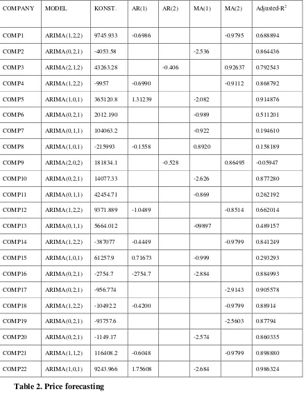
The testing of stock price prediction was done using the same steps as when testing hypothesis 1: performing a stationary test, searching for a tentative model and attempting forecast using the model obtained. Based on this analysis stage, a price forecasting model was obtained as shown in table 2 (Appendix)
To confirm the second hypothesis, the mean discrepancy between the actual value and the fitted value of the sample firms was tested. The two-mean average difference test yielded the following results: a significance value of 0.487, with alpha 0.05. Since this significance value was greater than alpha, the hypothesis that there time series price has the ability to predict future prices was statistically confirmed.
4. The ability of earnings to predict stock price fluctuation pattern (Testing of H3)
To examine the ability of time series profit to forecast patterns of stock price movement, we had to examine the correlation between the company's thorough earnings data and data on shares price. If the fluctuation pattern of earnings was similar to the fluctuating pattern of stock price rates, it could be concluded that the two data has a significant relationship, as would be indicated by the correlation value of the time series returns and the stock price series. If the correlation value was a significant positive, then it could be decided that time series profit could be used to predict stock prices. Using statistical tests, a correlation value of 0.167 with a 0.007 significance was obtained. Statistical analysis showed that the significance value of 0.007 was below 0.05 alpha, which meant that the hypothesis that time series profits has the ability to predict stock prices pattern was statistically supported.
5. The ability of time series cash flow to predict future cash flow (Testing of H4).
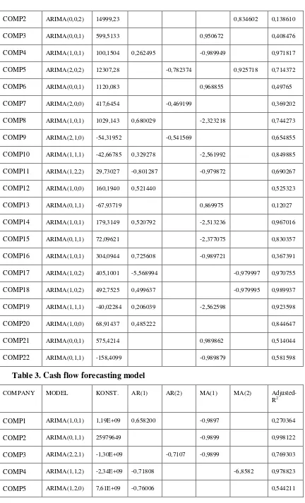
To test the ability of time series cash flow to predict future cash flow, the same steps were taken as those to prove hypothesis 1. From the analysis stage, a forecasting model was obtained, as shown in Table 3 (Appendix 1). The model obtained was then used for forecasting cash flow. To confirm the fourth hypothesis, the mean difference between the actual value and its fitted value of the sample companies was tested. The differential test results indicated that the two value’s mean discrepancy had a significance level is 0.873, which was to say that the difference was not significant. This meant that the 4thhypothesis presented, which says that time series cash flow has the ability to predict future cash flows, was confirmed.
6. The ability of cash flow to predict stock price fluctuation pattern (Testing of H5)
To examine the ability of time series cash flow to forecast stock prices fluctuation pattern we examined the correlation between a company’s data of cash flow and the company's stock prices. If the pattern of cash flows was similar to the fluctuation pattern of stock prices, then it can be concluded that the two data has significant relationship, as would be indicated by the significance value of the correlation. If the value of the correlation was significant, it can be decided that time series cash flows can be used to predict stock prices. Statistical analysis showed that the correlation value of the two data is 0.018 with a significance of 0.783, which was greater than 0.05 alpha. Therefore it was concluded that statistically, the fifth hypothesis, which stated that cash flow has the ability to predict time series stock prices fluctuation pattern, was not be supported.
D. Conclusion and Advice
1. Conclusion
This study aims to prove empirically the ability of earnings to predict future earnings and stock prices fluctuation patterns and to prove the ability of cash flow to predict future cash flow and stock price fluctuation pattern. A total of 22 samples were obtained with set criteria. Through statistical analysis, a model was obtained which would fit the use of forecasting profit, forecasting cash flow and forecasting patterns of stock prices movement.
Since statistical analysis showed a significance value of 0.007 below 0.05 alpha, then statistically, the third hypothesis which says that time series profit has the ability to predict stock prices pattern was confirmed.
The fourth hypothesis says that time series cash flow can be used to predict future cash flows. Differential test resulted in a significance level of 0.873, which meant that it had no significant discrepancy. This meant that the hypothesis that time series cash flow has the ability to predict future cash flows was statistically proven.
The fifth hypothesis states that cash flow has the ability to predict to fluctuation pattern of stock prices. If the pattern of cash flow was similar to the fluctuation pattern of stock prices, then it could be concluded that the two had a significant relationship as indicated by their correlation value. If the correlation value was significant, then time series cash flow could be used to predict stock prices. The statistical analysis, however, resulted in a correlation value of 0.018 and with 0.783 significance, which was greater than 0.05 alpha. Therefore it was concluded that statistically, the fifth hypothesis, which stated that time series cash flow has the ability to predict stock price fluctuation patterns, was not acceptable.
2. Advice
This study tests the ability of time series returns to predict future earnings and to predict stock price fluctuation pattern. This study also tests the ability of time series cash flows in predicting future earnings and future stock price fluctuation patterns. The results of the study may have been influenced by the purposive sampling, which therefore means that further researches can be done by extending the research sampling. This research has also not included into consideration other factors such as profit leveling or other financial information. Therefore, the following study is expected to consider factors that are thought to be able to predict earnings, cash flows and stock price pattern.
References
Ball, Ray, and Philip Brown, 1968. An Empirical Evaluation of Accounting Income Numbers. Journal of Accounting Research:159-178.
--- dan R. Watts, 1972. Some Time Series Properties of Accounting Income. Journal of Finance(June): 663-682 Baridwan, Zaki, 1999.Intermediate Accounting, BPFE, Yogyakarta.
………., 1997. Analisis Tambahan Informasi Laporan Arus Kas. Jurnal Ekonomi dan Bisnis Indonesia, Vol. 12:113.
Bernard, V. , et al., 1989. The Nature and Amountof Information in Cash Flows and Accrual. The Accounting Review, October: 624-652.
Bowen, et al., 1986, The Evidence on The Relationship Between Earnings and Various Measures of Cash Flow from Operation.The Accounting Review(LXI), 4,
713-Beaver, William H., 1970. The Time Series Behavior of Earnings. Supplement toJournal of Accounting Research: 62-69.
Brown, LD., 1993. Earnings Forecast Research: Its Implications for Capital Market Research, International and Business Research,14 Spring: 113-124.
Finger, Catherine A., 1994., The Ability of Earnings to Predict Future Cash Flow”, Journal of Accounting Research.Vol.32, No.32 (Autumn):210-223.
Fama, E., 1990. Stock returns, expected returns, and real activity,Journal of Finance45: 1089-1108.
Foster, George, 1986.Financial Statement Analysis,Second Edition, Prentice-Hall International.
---, 1977a. Quarterly Accounting Data: Time-series Properties and Predictive-Ability Result. Accounting Review,Januari: 1-21.
Fairfield, et al., 1996. Accounting Classification and The Predictive Content of Earnings,The Accounting Review, Vol.71, No.3 (July): 337-355
Hendriksen, Eldon S., dan Van Breda, 1991.Accounting Theory, Fifth Edition, Irwin United State of America. Hermawan, A. dan Nuranto Hadyansah, 2002. Analisa Pengaruh Format Metode Langsung Dalam Laporan Arus
Kas Terhadap Return Saham. Proceeding Simposium Nasional Akuntansi, September: 102-110.
Ismail, Badr E. dan Moon A. Kim, 1989. On The Association of Cash Flows Variables with Market Risk:Further Evidence. The Accounting Review, January: 125-136.
Ikatan Akuntan Indonesia, 2007.Standar Akuntansi Keuangan,Salemba Empat, Jakarta
Isgiyarta, Jaka, 1997. “Klasifikasi Akuntansi dan Kemampuan Prediksi Laba,”Tesis S2, Universitas Gadjah Mada. Kholidiah, 2002. Perbandingan Keakuratan Metode Naïve, Regresi Sederhana & Box-Jenkins,” Tesis, Tidak
Dipublikasikan, Universitas Gadjah Mada, Yogyakarta.
Kusuma, Poppy D. I., 2003. “Nilai Tambah Kandungan Informasi Laba dan Arus Kas Operasi”, Proceeding Simposium Nasional Akuntansi (SNA) VI, Surabaya (Oktober): 304-313.
Kuncoro, Mudrajad, 2001.Metode Kuantitatif: Teori dan Aplikasi untuk Bisnis dan Ekonomi, Edisi pertama, UPP AMP YKPN, Yogyakarta.
Lipe R.C., 1986. The Information Contained in The Components of Earnings, Journal of Accounti“Kemampuan Laba dan Arus Kas dalam Memprediksi Laba dan Arus Kas Perusahaan Go Publik di Indonesia”, Jurnal Riset Akuntansi Indonesia, Januari: 1-11.
Rayburn, J., 1986. “The Association of Operating Cash Flow and Accrual With Security Returns’, Journal of Accounting Research (Supplement): 112-133
Sugiri, S., 2003. “Kemampuan Laba Rincian untuk Memprediksi Arus Kas,” Desertasi, Tidak Dipublikasikan, Universitas Gadjah Mada, Yogyakarta.
Supriyadi, 1999. “The Prdictive Ability of Earnings Versus Cash Flow Data to Predict Future Cash Flows: A Firm Specific Analysis”,Gadjah Mada International Journal of Business, Vol.1, No.2, (September): 113-132. Sunariyah, 1996. “Ketepatan Ramalan Laba di Prospektus Pada Awal Penawaraan Umum di Pasar Modal
Indonesia,”Tesis, Tidak Dipublikasikan, Universitas Gadjah Mada, Yogyakarta: 1-89.
Utami, C. Dilah., 1999, “Muatan Informasi Arus Kas dari Aktivitas Operasi, Investasi, dan Pendanaan”, Jurnal Bisnis dan Akuntansi, No.1: 15-27.
Appendix:
Table 1. Earnings forecasting model
COMPANY MODEL KONST. AR(1) AR(2) MA(1) MA(2) Adjusted-R2
COMP1 ARIMA(1,2,2) 9745.933 -0.6986 -0.9795 0.688894
COMP2 ARIMA(0,2,1) -4053.58 -2.536 0.864436
COMP3 ARIMA(2,1,2) 43263.28 -0.406 0.92637 0.792543
COMP4 ARIMA(1,2,2) -9957 -0.6990 -0.9112 0.868792
COMP5 ARIMA(1,0,1) 365120.8 1.31239 -2.082 0.914876
COMP6 ARIMA(0,2,1) 2012.190 -0.989 0.511201
COMP7 ARIMA(0,1,1) 104063.2 -0.922 0.194610
COMP8 ARIMA(1,0,1) -215993 -0.1558 0.8920 0.158189
COMP9 ARIMA(2,0,2) 181834.1 -0.528 0.86495 -0.05947
COMP10 ARIMA(0,2,1) 14077.33 -2.626 0.877280
COMP11 ARIMA(0,1,1) 42454.71 -0.869 0.262192
COMP12 ARIMA(1,2,2) 9371.889 -1.0489 -0.8514 0.662014
COMP13 ARIMA(0,1,1) 5664.012 -09897 0.489157
COMP14 ARIMA(1,2,2) -387077 -0.4449 -0.9799 0.841249
COMP15 ARIMA(1,0,1) 61257.9 0.71673 -0.999 0.293293
COMP16 ARIMA(0,2,1) -2754.7 -2754.7 -2.884 0.884993
COMP17 ARIMA(0,2,1) -956.774 -2.9143 0.905578
COMP18 ARIMA(1,2,2) -10492.2 -0.4200 -0.9799 0.88914
COMP19 ARIMA(0,2,1) -93757.6 -2.5603 0.87794
COMP20 ARIMA(0,2,1) -1149.17 -2.574 0.860335
COMP21 ARIMA(1,1,2) 116408.2 -0.6048 -0.9799 0.898880
COMP22 ARIMA(1,0,1) 9243.966 1.75608 -2.684 0.986324
Table 2. Price forecasting
COMPANY MODEL KONST. AR(1) AR(2) MA(1) MA(2)
Adjusted-R2
COMP2 ARIMA(0,0,2) 14999,23 0,834602 0,138610
COMP3 ARIMA(0,0,1) 599,5133 0,950672 0,408476
COMP4 ARIMA(1,0,1) 100,1504 0,262495 -0,989949 0,971817
COMP5 ARIMA(2,0,2) 12307,28 -0,782374 0,925718 0,714372
COMP6 ARIMA(0,0,1) 1120,083 0,968855 0,49765
COMP7 ARIMA(2,0,0) 417,6454 -0,469199 0,369202
COMP8 ARIMA(1,0,1) 1029,143 0,680029 -2,323218 0,744273
COMP9 ARIMA(2,1,0) -54,31952 -0,541569 0,654855
COMP10 ARIMA(1,1,1) -42,66785 0,329278 -2,561992 0,849885
COMP11 ARIMA(1,2,2) 29,73027 -0,801287 -0,979872 0,690267
COMP12 ARIMA(1,0,0) 160,1940 0,521440 0,525323
COMP13 ARIMA(0,1,1) -67,93719 0,869975 0,12027
COMP14 ARIMA(1,0,1) 179,3149 0,520792 -2,513236 0,967016
COMP15 ARIMA(0,1,1) 72,09621 -2,377075 0,830357
COMP16 ARIMA(1,0,1) 304,0944 0,725608 -0,989721 0,367391
COMP17 ARIMA(1,0,2) 405,1001 -5,568994 -0,979997 0,970755
COMP18 ARIMA(1,0,2) 492,7525 0,499637 -0,979995 0,989937
COMP19 ARIMA(1,1,1) -40,02284 0,206039 -2,562598 0,923598
COMP20 ARIMA(1,0,0) 68,91437 0,485222 0,844647
COMP21 ARIMA(0,0,1) 575,4214 0,989862 0,514044
COMP22 ARIMA(0,1,1) -158,4099 -0,989879 0,581598
Table 3. Cash flow forecasting model
COMPANY MODEL KONST. AR(1) AR(2) MA(1) MA(2)
Adjusted-R2
COMP1 ARIMA(1,0,1) 1,19E+09 0,658200 -0,9897 0,270364
COMP2 ARIMA(0,1,1) 25979649 -0,9899 0,998122
COMP3 ARIMA(2,2,1) -1,30E+09 -0,7107 -0,9899 0,769303
COMP4 ARIMA(1,1,2) -2,34E+09 -0,71808 -6,8582 0,978823
COMP6 ARIMA(1,0,1) -2044585 0,735484 -0,98967 0,536350
COMP7 ARIMA(0,1,1) -9,26E+09 -0,9895 0,486128
COMP8 ARIMA(2,1,2) -1,26E+09 -0,36971 2,4122 0,886184
COMP9 ARIMA(0,0,2) 2,58E+10 -0,8726 0,409488
COMP10 ARIMA(1,1,2) 1,27E+09 -0,73184 -0,9799 0,564690
COMP11 ARIMA(0,2,2) -1,16E+10 -0,980 0,814279
COMP12 ARIMA(0,0,2) 4,15E+09 0,93158 0,735015
COMP13 ARIMA(0,0,2) 2,33E+09 0,9385 0,746383
COMP14 ARIMA(1,2,2) -4,56E+09 -0,68332 -0,98 0,694898
COMP15 ARIMA(1,1,2) 2,11E+09 -0,82789 -0,9799 0,651780
COMP16 ARIMA(1,1,2) -20802338 -0,838933 -0,979785 0,635361
COMP17 ARIMA(1,1,2) -5,20E+09 -0,690656 -0,979458 0,763598
COMP18 ARIMA(2,0,2) 2,27E+08 0,017228 2,188483 0,995381
COMP19 ARIMA(1,1,2) -5,42E+08 -0,656211 -0,884427 0,371667
COMP20 ARIMA(0,1,1) -3,22E+09 -0,989436 0,544668
COMP21 ARIMA(1,2,2) 1,32E+08 -0,498928 -0,97999 0,755118