WATER SURFACE RECONSTRUCTION IN AIRBORNE LASER BATHYMETRY FROM
REDUNDANT BED OBSERVATIONS
G. Mandlburgera,∗, N. Pfeiferb, U. Soergela
a
University of Stuttgart, Institute for Photogrammetry, Stuttgart, Germany - (gottfried.mandlburger, uwe.soergel)@ifp.uni-stuttgart.de b
TU Vienna, Department of Geodesy and Geoinformation, Vienna, Austria - [email protected]
Commission II, WG II/10
KEY WORDS:LiDAR bathymetry, water surface reconstruction, air-water-interface, water bottom topography, refraction correction
ABSTRACT:
In airborne laser bathymetry knowledge of exact water level heights is a precondition for applying run-time and refraction correction of the raw laser beam travel path in the medium water. However, due to specular reflection especially at very smooth water surfaces often no echoes from the water surface itself are recorded (drop outs). In this paper, we first discuss the feasibility of reconstructing the water surface from redundant observations of the water bottom in theory. Furthermore, we provide a first practical approach for solving this problem, suitable for static and locally planar water surfaces. It minimizes the bottom surface deviations of point clouds from individual flight strips after refraction correction. Both theoretical estimations and practical results confirm the potential of the presented method to reconstruct water level heights in dm precision. Achieving good results requires enough morphological details in the scene and that the water bottom topography is captured from different directions.
1. INTRODUCTION
Laser scanning is a polar 3D measurement method. Starting with the exterior orientation of the sensor coordinate system, and us-ing the polar measurements of range and direction, the 3D tar-get point coordinates are computed. Laser bathymetry is an opti-cal two media measurement method. While the sensor is in one medium, the target (point) is in another. The interface surface between the two media either needs to be known in advance or determined during the measurement in order to correct the raw 3D point coordinates due to refraction at the interface and differ-ent signal velocity in air and water (Gudiffer-enther et al., 2000).
In the ideal case, the sensor records two echoes, one from the air-water interface and one from the bottom of the air-water body. The received signal strength of the water surface reflection mainly de-pends on the local incidence angle and the loss of transmission through the surface (Abdallah et al., 2012; Guenther, 1986). Dy-namic water surfaces caused by wind induced capillary waves or gravity waves exhibit a high degree of diffuse reflection, which generally results in good water surface return coverage. In con-trast, specular reflection is dominating for very smooth water sur-faces and can lead to laser echo drop outs. This is especially the case for modern topo-bathymetric sensors featuring a rela-tively small laser footprint diameter of typically less then 1m (Fernandez-Diaz et al., 2016; Pfennigbauer et al., 2011).
Literature on water surface mapping based on laser scanning fo-cuses on direct observation of interface reflections. This espe-cially applies to the field of laser bathymetry, where either data from the green wavelength alone (Pfennigbauer et al., 2011) or from both green and near infrared wavelengths (Thomas and Guenther, 1990; Guenther et al., 1994; Hilldale and Raff, 2008; Kinzel et al., 2013) are used, but also to topographic laser scan-ning from both manned and unmanned aerial platforms (H¨ofle et
∗Corresponding author
al., 2009; Mandlburger et al., 2015b), and even terrestrial laser scanning (Streicher et al., 2013). To our best knowledge, no in-direct methods for reconstructing water level heights exist in the field of laser scanning in general, and laser bathymetry in partic-ular.
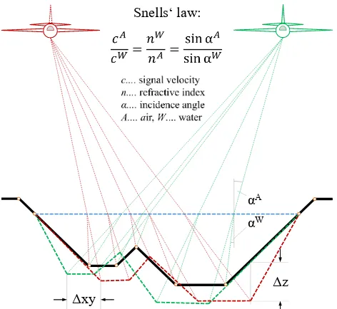
We are, therefore, investigating the case of multiple observations of the same bottom surface of a water body by laser bathymetry. Observing the same surface repeatedly from different view points provides over-determination, i.e. redundancy. The question arises if this redundancy can be used to reconstruct both the river bot-tom surface and the air-water interface. In this contribution we assume that the sensor system is already geometrically calibrated, i.e. the exterior orientation of the sensor coordinate system is known for the entire flight path. Each polar measurement in-cludes a direction and a time measurement. The emitted laser signal passes through the medium air, is refracted at the air-water interface, passes through the medium water, is reflected at the bot-tom surfaces, and finally travels the same way back to the sensor. The round-trip travel time along the refracted ray is measured. We further assume that measurements are recorded at least from two distinct viewpoints.
Δxy
Δz αA
αW
Snells‘ law:
Figure 1. Schematic diagram of redundant bed observations from different view points. Due to beam refraction at the air-water-interface (blue dashed line) the uncorrected profiles
(green and red dashed lines) are displaced in horizontal and vertical direction against the true water bottom (black solid line).
The remainder of the manuscript is structured as follows: The theory is detailed in Section 2 and in Section 3 the study area and a practical water surface reconstruction work-flow are presented. The results are discussed in Section 4 and the findings as well as future work are summarized in Section 5.
2. THEORY
To study the problem, a simplified mathematical model is built (cf. Figure 2). The origin of the laser’s coordinate system is de-noted byoi, the direction of the ray isviA, a unit vector. The
su-perscriptAdenotes the medium air, whileWdenotes the medium water. Additionally, the (one way travel) time is given astA+W
. Given are also the speed of light in aircA
and watercW
. The rel-ative refraction index is denotednW
A =c
A/cW
, which is around 1.33. In order to determine the air-water interface surface along the ray, the time measurement needs to be split into its two com-ponents:1
tA+W=tA+tW (1)
Under the assumption of a horizontal and static air-water inter-face surinter-face, the ray direction unit vector in the water is computed as:
The right hand side vector in Eq. 2 is normalized (subscript 0) in order to makeviWa unit vector, too.
2.1 Water level from the vertical component
Assuming that the ground is (locally) horizontal, its elevation is the unknowngzand the unknown height of the water column is
1Note, that in this theory section it is assumed that the signal is always
traveling through air and through water. With other words, only “wet” points are considered.
Figure 2. Schematic drawing observing ground reflections in constant water depthwfrom two different viewing directions.
The pointgA+Wi is the point without refraction correction.
w(cf. Figure 2). The travel time in water and the water height are then related by:
Under the assumptions above, the ground pointgiis determined
from the polar measurements using Eqs. 1, 2, and 4:
gi = oi+vAit
The scalar product of the vectors(0 0 −1)and vWi provides
the vertical component of the propagation direction of the ray. In photogrammetric and laser scanning terminology, Eq. 6 gives the under-water object point coordinates in function of the exterior orientation, scan angle, (one-way) travel time, and height of the water columnw.
Measuring the ground points with the elevationgz from two or
more positions, an observation equation with the residualeican
be set up:
Given two observations,i= 1,2a unique solution can be found, if it exists (cf. Figure 2). For more observations, a solution can be found by minimizing the residualsei. The unit of the residuals
is the same as of the ground elevationgz, thus meter. A
differ-ent off-nadir directionsviAleading to differentvWi are required.
This is, however, not fulfilled for most airborne laser bathymetry instruments with a circular scan pattern (Palmer scanner) aim-ing at a constant incidence angle between laser beam and water surface of20◦. The approach of different view points for observ-ing a horizontal ground and air-water interface, i.e. showobserv-ing no features in planimetry, is thus, only feasible for instruments pro-viding enough incidence angle variation (Fernandez-Diaz et al., 2016).
Using Eq. 8 can – nonetheless – be studied to understand the accuracy potential of this method. The first term, the constant part, is the polar point determination neglecting the two media case (seegA+Wi in Figure 2). In the second term, the coefficient
ofwis the correction for the water column. For different angles of incidence (i.e. off-nadir angles for a horizontal water surface), the corrections forw=1 m are given in Table 1.
Angle[◦] horizontal offset[m/m] vertical offset[m/m]
Table 1. Correction coefficients for horizontal and vertical direction for different angles of incidence.
Considering the angles of10◦ and20◦, the difference in verti-cal correction (0.321-0.296 m/m) amounts to 2.5 cm for a water column of 1 m, thus a factor of 40. If time measurement allows a determination of the elevation with an accuracy in the order of 2 cm, this would allow determining the water column with an ac-curacy in the order of 80 cm.
The table also shows that the variation of the correction in the lat-eral direction is much higher. What is more, and does not show up in the table but can be seen in Figure 1, is that the horizontal coefficient changes its sign when looking from opposite direc-tions. This results in an even larger horizontal displacement of the same spot viewed from opposing directions (e.g. forward and backward look for standard20◦circular scans patterns).
2.2 Water level from the horizontal component
In a second approach we are thus still assuming a horizontal air-water interface, but in addition a feature on the ground which can be identified in two laser scans over the same area, i.e. like a corresponding point in forward intersection. This could be a geo-metrical feature, e.g. a peak-like local maximum in elevation, or a radiometric feature, e.g. a bright spot among low energy returns. A similar analysis as above, using only the horizontal component, shows that the water height is affected by a factor 2.5 in respect to a horizontal displacement of one unit. Given a horizontal po-sitioning accuracy (of the peak) of 20 cm thus leads to a vertical accuracy of the water height of 50 cm.
As identification of point like features is not the typical case in airborne laser bathymetry, this ‘peak’ will be replaced by surfaces with differently oriented normal vectors. Examples of features fulfilling the above criterion are large submerged boulders or lo-cal depressions (pools). This makes the unknown ground model considerably more complex. The water column does not have
w
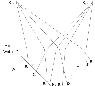
Figure 3. Schematic drawing of observing two opposing, constantly sloped banks with laser bathymetry from two scan positions. Measurements 1–4 come from one scan, 5–8 from the
second scan. The measurements 1, 2, 5, 6 are on the left faceL
and 3, 4, 7, 8 on the right faceR.
a constant height anymore, andwis re-interpreted as the water levelw, which is a co-ordinate as, e.g.,ozorgz, and denotes the
distance from the reference surface of elevation. The water depth is thusw−gz. In a first instance, the pointgi = (gx,i, gz,i)is
computed according to Eq. 5:
gi=oi+vAit
The formulation has the problem thatgi depends on the water
depth, which is varying and not a constant as above. Thus, the al-ternative of computing the point position using under-water con-ditions and adding a correction for the part in the air is pursued.
oz,i−w = (0 0 −1)vAit
More precisely, the pointgiis computed using the under-water
direction and speed for the entire measured timetA+Wi , which
is then adjusted by the entire correction for air conditions from the origin down to the reference surface, of which the correction from the water level down to the reference surface is again sub-tracted. As above, if the position of the platformoiis known, the
directions of the beam above and below the water surfaceviAand vWi and the corresponding speeds of lightcAandcWare known,
and the (one way) travel time of the signaltA+W
i is observed, the
only unknown is the horizontal, static water levelw.
on the profile from two scan positions, thus eight time measure-ments in total. This leads to a redundancy of 3. The equations for the faces arez=kx+d, with unknown slopekand offsetd. The observation equations are:
ei=kSgx,i+dS−gz,i , S∈ {L, R}, i . . .point nr. (14)
Inserting Eq. 13 into the equation observations of the two faces, Eq. 14, leads to a bilinear system in the unknowns
kL, dL, kR, dR, w.
Running a simulated example confirms the convergence of the equation system. Using the normal equation inverse, the preci-sion ofwcan be estimated. With slopes in the order of 30%, an inclination angle of the rays of20◦, and a regular spacing of 8 points over a profile length of 8 m, the precision inw is ap-prox. the 8-fold of the measurement precision. Thus, if range (or height) measurement is accurate to 3 cm, the water level will be estimated with a precision of 25 cm. An error of this size in the water level leads to an error of 8 cm in the height of the water bottom point.
2.3 Forward modeling
The equations presented in the above subsections allow an in-version and determination of an optimal water level by solving a least squares (optimization) problem. The formulae were short because of the horizontal static water level and the simple model for the ground surface. Forward modeling, on the other hand, al-lows determining the river bottom points assuming a certain wa-ter levelwin Eq. 13 for arbitrary ground surface profiles, and the shape deviation this level causes on profiles.
For moderate slopes and typical inclination angles in laser bathymetry, the ground will always be estimated too high if the water level is assumed too high. In Table 1 the ratio of changes in lateral profile position and in height is given, for correction from air to water propagation. For a certain inclination angle, e.g.20◦, this gives the direction of the correction vector. If the ground gra-dient vector has the same direction as this correction vector, then this sloped ground will be mapped onto itself, and not shifted up-wards. For the case of20◦this means, that ground below water with an inclination of56◦, or 149% slope, will not be shifted up-wards. For horizontal ground, the upward shift will be 22 cm for a water level that is 1 m too high (and not 30 cm, as the correc-tion is defined via 1 m vertical travel distance in water and not in air). If the ground was even steeper (a rather theoretical case), the wrongly determined ground would be shifted to a position below the real ground. If the viewing direction and the ground gradient direction are opposing each other, in the sense that one is point-ing left and the other is pointpoint-ing right of the vertical (or the water surface normal), then the slope is always shifted upwards, if the water level is assumed too high. In general it can be said that the vertical shift of inclined ground due to a wrong water level is higher for the slope that faces the laser sensor than for a slope that is (more) aligned with the beam direction.
Figure 4 demonstrates the above with an example. It shows ground that is inclined with 25%, followed by a horizontal section and a small geometric feature. The different lines indicate hypo-thetical profile positions assuming different water levels, and the gray line corresponds to the correct water level, and thus to the correct position of the points on the ground. For different values of a wrongly assumed water level and for observation positions to the left and to the right of this profile, the effect on the recon-structed ground surface is shown. For the 25% slope and20◦
Figure 4. Deformation [m] of the water bottom from its ideal position depending on incorrectly assumed water level and viewing position. Gray: ground for the correct water level, red/green: water level 0.3/1.0 m too high (solid) or too low
(dashed), bright/pale: view position on the left/right.
off-nadir viewing direction and a water level that is 30 cm too high, the sloped surface is reconstructed 6 cm too high if viewed from the left, and 8 cm too high if viewed from the right. The difference in upward shift is thus 2 cm. This shift occurs not only at a point but systematically along the entire slope. The upward shift in the horizontal section is 7 cm, but equal for the left and the right view. The apparent horizontal displacement caused by the small feature, which is found at the end of the profile, is about 9 cm.
3. MATERIALS AND METHODS
The theoretical derivation included a number of assumptions which do not apply strictly in the practical context of an airborne laser bathymetry measurement over a ‘real’ waterbody. Thus, a proof of concept in a real-world context can, to some extent, verify the theoretical derivation, but especially identify the ad-missibility of the idealization and guide further refinement. In the following subsections we therefore present the study area and the details of a laser bathymetry data acquisition serving as basis for two experiments. In the first experiment we derive strip-wise uncorrected river bottom surfaces and evaluate strip-wise height differences for water levels deviating from the correct water level. In a second experiment the task is reversed to find the best water level from the analysis of the height differences.
3.1 Data acquisition
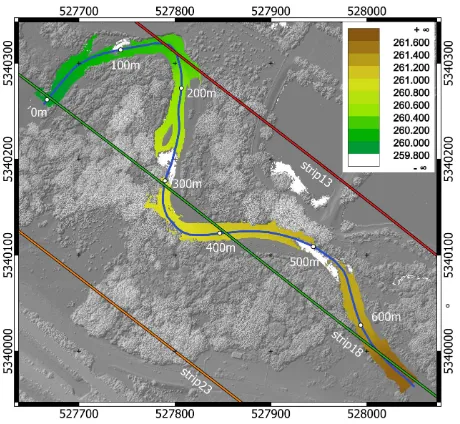
Figure 5. Study area Neubacher Au (Pielach River, Austria); river axis: blue line; flight trajectories: red, green, and orange
lines; water level heights: color coded raster map (only areas with sufficient returns from the IR channels are displayed);
image background: shaded relief map superimposed with gray-scale encoded surface elevations.
Data acquisition was carried out with theRIEGLVQ-880-G topo-bathymetric laser scanner mounted in the nose pod of a Diamond DA42 light aircraft from 600 m above ground level on June, 16, 2016. The sensor uses a green laser (λ=532 nm) for measuring the bathymetry and the riparian topography and an (optional) in-frared laser (λ=1064 nm) to acquire additional echos from the air-water-interface. Whereas a rotating multi-facet prism is used for the IR channel to scan the terrain and the water surface below the aircraft in parallel profiles perpendicular to the flying direc-tion, the green signal is deflected via an inclined rotating mir-ror (Palmer scanner) resulting in a circular scan pattern on the ground. The vendors’ processing software separates the measure-ments of the green laser into a forward and a backward looking semicircle.
From the entire flight block a 680 m reach (cf. blue line in Fig-ure 5) was analyzed in detail. The three flight strips covering the area of interest provide six different semicircular datasets and, thus, viewing directions. All combinations of overlapping datasets were used to estimate the water level heights from pair-wise redundant river bed measurements as described in Sec-tion 3.3. The water surface returns from the IR channel were used as reference (i.e. ground truth) for assessing the accuracy of the water level estimation. From all IR reflections a Digital Watersurface Model in regular grid structure (grid width=50 cm) was derived.
3.2 Experiment 1
The first experiment aims at demonstrating the feasibility of de-riving the air-water interface via redundant observations of the bottom topography based on real-world data. We show that the minimum strip-to-strip height differences are in fact obtained when using the correct water surface model, whereas vertically shifted variants show higher discrepancies.
In a first step, the ground and water bottom points are identi-fied as the method relies on redundant observation of the
station-ary bottom surface. This is carried out for each strip separately based on the uncorrected echoes of the green laser channel. From the resulting ground points a Digital Terrain Model (DTM) is derived with moving least squares interpolation and stored as a regular 0.5 m grid. Points located on horizontal surfaces are sub-sequently identified by estimating local surface normal vectors and only points on slanted surfaces (river bank, submerged fea-tures) are considered for further analysis, as horizontal areas do not add relevant information for water surface reconstruction (cf. Figure 4).
For verifying the feasibility of the approach, the water surface is reconstructed from all IR interface returns and serves as reference for the validation later on. Using the semi-automatic approach described in Mandlburger et al. (2015a), an approximated Digital Water-level Model (DWM) is first generated based on linear wa-ter surface profiles. A refined DWM (50 cm grid) is inwa-terpolated from all IR echoes within a small height tolerance band around the approximate model. It is noted that the described procedure does not lead to a horizontal water level, but features (i) the wa-ter level drop along the river course, (ii) occasional tilting of the water surface perpendicular to the flow directions at point bars, and (iii) local water surface irregularities due to waves caused by submerged boulders or dead wood.
The determined water surface model is then shifted in 10 cm steps both below and above the water table to a maximum offset of
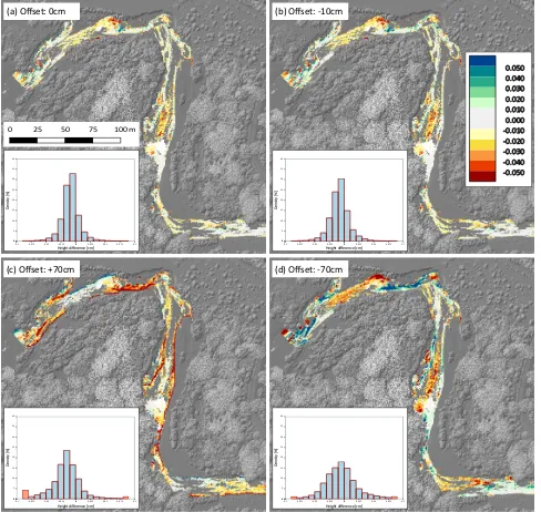
±70 cm. Range and refraction correction is subsequently carried out for each strip separately and for each of the resulting artificial water surface models. For each offset level, strip-wise DTMs are interpolated from the corrected laser points and pair-wise height difference models are derived for any overlapping strip combina-tion. The results for strip pair 13/18 are illustrated in Figure 6 and discussed in detail in Section 4.
3.3 Experiment 2
In a second experiment the problem is reversed to find the local water level height by analyzing the vertical deviations. For run-ning waters we propose the following strategy. For the sake of simplicity we neglect a potential water level tilt as well as water surface roughness (i.e. waves). For each strip of an overlapping strip pair we select all ground/bottom points within a user defined range along and across the river axis individually. The across track extent of the selection polygon should hereby be chosen to cover the entire wetted perimeter and the adjacent riparian area. The along track extent mainly depends on the ground/bottom point density and should be chosen to allow statistical analysis (e.g.>1000 points). Refraction correction is then carried out us-ing the mean elevation of the selected points as startus-ing level. The water level is then shifted upwards and downwards in user defined intervals (e.g. 5 cm) and the point-to-plane distances between the corrected strip point clouds are calculated. The procedure is re-peated until a minimum deviation is reached. For the minimum search different statistical measures are investigated. These are: (i) inter decile range (IDR, i.e. q90-q10), (ii) inter quartile range (IQR, q75-q25), (iii) q40-q60-range (q60-q40), (iv) standard de-viation (stdev), and (v) robust standard dede-viation (σM AD, median
absolute deviation).
4. RESULTS AND DISCUSSIONS
(c) Offset: +70cm (d) Offset: -70cm
Height difference [cm]
0 0.025 0.05 0.075 0.1
Height difference [cm] 0 0.025 0.05 0.075 0.1
Height difference [cm]
0 0.025 0.05 0.075 0.1
Height difference [cm]
0.050
Figure 6. Color coded height differences between strips 13 (channel 1) and 18 (channel 1) derived from points classified as ground after refraction correction based on the correct (a) and vertically shifted water surface models (b, c, d). Image background:
superimposition of DSM heights and shaded relief derived from IR channel.
the correct water level was used and the impact of a shifted wa-ter level on the strip height differences was explored. The plots and histograms shown in Figure 6 confirm that (i) the global de-viations are smallest when using the correct water level and (ii) measurable differences are obtained compared to the results using incorrect water surface heights. The histogram of height differ-ences corresponding to the correct water level (Figure 6a) shows the highest mode, i.e. 33% of the data, as well as the thinnest tails in the distribution of height differences.
The offset of -10 cm leads to a similar histogram compared to the correct water level, thus indicating the sensitivity of the ap-proach. For offsets 70 cm, above and below, the tails of the dis-tribution are notably thicker, but also the values around zero are more dispersed. We consider this result a proof of concept that water surface reconstruction from redundant bed observation is generally feasibly, not only in theory but also in a practical
con-text. The obtained uncertainties are in line with the theoretical height error estimates presented in Section 2.2.
This result stimulated the second experiment where local water level heights were estimated from pair-wise overlapping river bed point clouds based on statistical analysis of the height residuals after refraction correction in different water levels. The 680 m long river reach was divided into (a) 10 m or (b) 20 m segments with a 20% overlap between the individual segments. For each section a representative water level was estimated. Although the inherent assumption of a locally horizontal water surface neglects a potential tilt of the actual water surface, we regard this simple model as sufficient for the intended proof of concept.
es-100m
height difference [m]
Histogram: q40-q60-range (20m sec�ons, submerged pts)
#Data: 41019
height difference [m]
Histogram: q40-q60-range (20m sec�ons, all points)
#Data: 41019
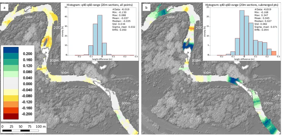
Figure 7. Deviations of modeled water surfaces from the reference water level derived from IR channel. (a) DWM derived from q40-q60-range for 20 m sections; (b) as (a) with statistics based on submerged points only.
strippair stdev σM AD IDR IQR q40-60
G13-0/G13-1 25 10 25 15 -00
G13-0/G18-0 -20 -15 -10 05 -05
G13-0/G18-1 -10 50 20 20 45
G13-0/G23-1 -00 10 -00 15 10
G13-1/G18-0 -10 -05 -00 -15 35
G13-1/G18-1 25 -05 25 05 45
G13-1/G23-1 25 25 10 40 40
G18-0/G18-1 -15 -15 -00 -00 -25
G18-0/G23-1 50 10 35 20 05
G18-1/G23-1 -10 25 -00 05 10
mean 06 09 10 11 16
rms 23 21 17 18 28
Table 2. Nominal-actual comparison of all strip pair combinations and all tested statistics in [cm] for section 165
timation as outlined in Section 3.3 and the rows denote the re-spective strip pair. Ghereby stands for the green laser channel followed by the strip number (two digits) and the suffix 0 or 1, respectively, denoting the forward or backward looking semicir-cle of each scan. Section 165 contains 10 overlapping strip pair combinations. For each strip pair and each statistical measure a water level height was estimated and compared to the refer-ence height (260.25 m) obtained from the IR channel. As can be seen from Table 2, there is no clear best choice, neither con-cerning the statistic nor w.r.t. the strip pair. A correct estimate can, for instance, be achieved from the standard deviation of pair G13-0/G23-1, the inter decile range of pair G13-1/G18-0, the in-ter quartile range of pair G18-0/G18-1, the q40-60 range of pair G13-0/G13-1, and the mode of pair G13-1/G18-0 (not shown in the table). Whereas the dispersion (rms: 17-28 cm) corresponds to the theoretical error estimates, on average all statistics show a positive bias for section 165 (mean: 6-16 cm).
As stated in Section 2, the success of the method depends on the (i) availability of morphological details and (ii) the viewing ge-ometry. Thus, the individual strip pairs are not equally distinctive for deriving water level heights via statistical analysis of height residuals. Consequently, the additional redundancy provided by
multiple strip pairs was further exploited by choosing the opti-mum water level height from the strip pair with the clearest min-imum distinctness. For each statistic the local water level was selected from the strip pair showing the lowest value of all avail-able strip pairs. The corresponding results for the entire reach, derived from the q40-q60 range metric, are displayed in Figure 7. Although other metrics like IQR andσM ADresulted in smaller
mean absolute errors, this metric was chosen because it was least prone to outliers (i.e. large height deviations from the reference water surface).
The color coded maps in Figure 7 show the deviations of modeled DWMs compared to the reference model. As stated earlier, the reference water surface model was obtained from the IR water surface returns. The modeled surfaces, in turn, are interpolated from the estimated water level heights along the river axis using the approach described in Mandlburger et al. (2015a). Potential tilts of the water surface perpendicular to the flow direction are hereby neglected. The errors committed by this simplification were estimated by analyzing the areal differences between the reference water surface model and a DWM constructed from hor-izontal profiles (i.e. z of profile = z at river axis). The deviations are negligibly small (rms: 1 cm) with maximum deviations of
±6 cm in backwater areas and areas with turbulent flow. DWM reconstruction from horizontal profiles perpendicular to the flow direction is therefore admissible for the study area and data cap-ture at hand.
the entire 680 m reach with maximum deviations of -15.0 cm and +8.8 cm, respectively. The rms of 5 cm is far better than expected from the theoretical error estimations. A possible reason for this rather low dispersion value is the fact that 6 overlapping datasets were available, resulting in a maximum of 15 overlapping pairs. Whereas such high strip overlaps are unlikely in the context of practical mapping projects, it led to errors below the expected level in our experiment.
While the variant using all section points yielded good results, us-ing only the submerged points would be more appropriate. This variant, however, shows larger errors in all metrics but the me-dian (min: -16.8 cm, max: +34.7 cm, rms: 9.4 cm, +2.7 cm). The volatility of the two variants clearly reveals the limits of the pro-posed estimation procedure. Still, we conclude that also the sec-ond experiment proofs the general feasibility of deriving water levels from redundant bed observations.
5. CONCLUSIONS AND OUTLOOK
In this contribution we investigated the feasibility of deriving wa-ter surface level heights from redundant observations of the wawa-ter bottom in laser bathymetry. Both theoretical reasoning and prac-tical experiments confirmed that indirect water surface determi-nation is possible provided that: (i) the water bottom is captured from at least two different positions, (ii) a static water surface can be considered for the entire data capturing period, (iii) the water surface can be locally approximated with planar or even horizon-tal models, (iv) horizonhorizon-tal and low textured water bottom sections are captured with different incidence angles, and (v) enough sub-merged features like boulders, tilted slopes, (gravel) bars, etc. are available for scanners utilizing a constant off-nadir angle over the entire (circular) scan line. Theoretical sensitivity analysis of a standard scenario (20◦off-nadir scan angle, 30◦bank slope, 3 cm laser ranging precision, locally horizontal water surface) resulted in a potential height accuracy of 25 cm.
Building on the theoretical findings, a practical experiment was carried out using a topo-bathymetric acquisition of the pre-alpine Pielach River (Austria) in June 2016. A water surface reconstruc-tion procedure was implemented based on statistical analysis of height differences between overlapping strip pairs after range and refraction correction of hypothetical water levels. The obtained air-water interface heights were compared to a reference model derived from surface echoes of the IR laser channel. The resid-uals showed an error (rms) of approx. 10 cm. Due to high re-dundancy provided by the very dense array of flight lines (strip overlap 75 %), the error is even smaller than expected from the theoretical error estimation. On the other hand, maximum errors of about±35 cm leading to bottom height errors of 12 cm were observed locally, especially in very shallow and flat sections lack-ing enough morphological details for precise water surface recon-struction from redundant water bottom observations.
We demonstrated the feasibility of a novel approach for water surface reconstruction. Considering realistic topo-bathymetric data capturing scenarios, the achievable height accuracy cannot compete with direct water level observations from reflections of near infrared or even green laser pulses at the air-water interface. However, the presented indirect reconstruction method can close data gaps in areas with no surface returns. This is especially valu-able for small footprint scanners hitting very smooth water sur-faces where laser echo drop outs are likely due to the high degree of specular reflection.
ACKNOWLEDGEMENTS
This work was funded by the German research foundation (DFG) project ’Bathymetrievermessung durch Fusion von Flugzeu-glaserscanning und multispektralen Luftbildern’. We gratefully acknowledge the contributions of Julia Bulat in generation of the sketches during her ‘university days for pupils’.
References
Abdallah, H., Baghdadi, N., Bailly, J., Pastol, Y. and Fabre, F., 2012. Wa-LiD: A New LiDAR Simulator for Waters. IEEE Geosci. Remote Sensing Lett., 9(4), pp. 744–748.
Fernandez-Diaz, J. C., Carter, W. E., Glennie, C., Shrestha, R. L., Pan, Z., Ekhtari, N., Singhania, A., Hauser, D. and Sartori, M., 2016. Capability Assessment and Performance Metrics for the Titan Multispectral Mapping Lidar. Remote Sensing, 8(11), pp. 1–33.
Guenther, G. C., 1986. Wind And Nadir Angle Effects On Air-borne Lidar Water Surface Returns. In:Proc. SPIE, Vol. 0637, pp. 277–286.
Guenther, G. C., Cunningham, A. G., Laroque, P. E. and Reid, D. J., 2000. Meeting the accuracy challenge in airborne lidar bathymetry. In:Proceedings of the 20th EARSeL Symposium: Workshop on Lidar Remote Sensing of Land and Sea, Dresden, Germany.
Guenther, G. C., LaRocque, P. E. and Lillycrop, W. J., 1994. Mul-tiple surface channels in Scanning Hydrographic Operational Airborne Lidar Survey (SHOALS) airborne lidar. In: Proc. SPIE, Vol. 2258, pp. 422–430.
H¨ofle, B., Vetter, M., Pfeifer, N., Mandlburger, G. and St¨otter, J., 2009. Water surface mapping from airborne laser scanning using signal intensity and elevation data. Earth Surface Pro-cesses and Landforms, 34(12), pp. 1635–1649.
Hilldale, R. C. and Raff, D., 2008. Assessing the ability of air-borne LiDAR to map river bathymetry. Earth Surface Pro-cesses and Landforms, 33(5), pp. 773–783.
Kinzel, P. J., Legleiter, C. J. and Nelson, J. M., 2013. Mapping River Bathymetry With a Small Footprint Green LiDAR: Ap-plications and Challenges. JAWRA Journal of the American Water Resources Association, 49(1), pp. 183–204.
Mandlburger, G., Hauer, C., Wieser, M. and Pfeifer, N., 2015a. Topo-Bathymetric LiDAR for Monitoring River Morphody-namics and Instream Habitats-A Case Study at the Pielach River.Remote Sensing, 7(5), pp. 6160–6195.
Mandlburger, G., Pfennigbauer, M., Riegl, U., Haring, A., Wieser, M., Glira, P. and Winiwarter, L., 2015b. Comple-menting airborne laser bathymetry with UAV-based lidar for capturing alluvial landscapes. In: Proc. SPIE, Vol. 9637, pp. 96370A–96370A–14.
Pfennigbauer, M., Ullrich, A., Steinbacher, F. and Aufleger, M., 2011. High-resolution hydrographic airborne laser scanner for surveying inland waters and shallow coastal zones. In: Proc. SPIE, Vol. 8037, pp. 803706–803706–11.
Streicher, M., Hofland, B. and Lindenbergh, R. C., 2013. Laser Ranging for Monitoring Water Waves in the new Deltares Delta Flume.ISPRS Annals of Photogrammetry, Remote Sens-ing and Spatial Information Sciences, II-5/W2, pp. 271–276.
![Figure 4. Deformation [m] of the water bottom from its idealposition depending on incorrectly assumed water level andviewing position](https://thumb-ap.123doks.com/thumbv2/123dok/3672781.1804421/4.595.307.539.70.231/figure-deformation-idealposition-depending-incorrectly-assumed-andviewing-position.webp)