DETERMINANT OF CHILD SCHOOLING IN INDONESIA Oleh: Losina Purnastuti
(Staf Pengajar FISE Universitas Negeri Yogyakarta) Abstract
Using the 1993 Indonesia Family Life Survey, this paper examines school participation among boys and girls in Indonesia and investigates why parents are less likely to keep their daughter in school. The analysis is based on indicators of school attendance. In particular we focus on the gender difference in school attendance, effect of parents’ education and employment, household resource constraint, location of the household and quality of the school. This paper finds significant gender differences in children’s education. Parents are more likely to send their sons to school rather than their daughters. Parents’ education has significant positive impact on their children’s schooling in different manner. Mothers’ education has stronger impact on girls’ school attendance, while fathers’ education has stronger impact on boys’ school attendance. Household income matters only for girls; it implies that girls belonging to poor families are less likely to go to school, and education is a luxury good for these girls. Further the number of children under 5 years old in the household also matters only for girls. This indicates that for girls there is a trade off between being in school and taking care of younger siblings as well as substituting for the mother in doing domestic tasks.
Keywords: Children’s schooling, gender differences, unitary model, Indonesia
A. Introduction
schooling; Millimet (2003) examines the effect of household size on human capital investment in children.
While recent literature documents the importance of children’s education in general, lately many researchers have focused on a more specific question – gender disparities in education. Schultz (2001) claims that the health and the schooling of children are more closely related to their mother’s education than father’s. Ahmed et al (2001) conclude that gender inequality in education may prevent a reduction of child mortality and fertility. It also slows the expansion of education on the next generation. In addition, it may be the case that gender inequality may hamper economic growth. Thus this evidence triggers an influx of studies on gender differences in education.
Many studies have been done in this area including; Tansel (1998), whose study indicates that both boys’ and girls’ schooling were found to be strongly related to their parent’s education and the parental education effects were larger on girls’ than on boys’ schooling. Kambhampati and Pal (2000) show that in terms of the predicted probabilities of no schooling, generally boys have a higher probability of going to school compared to girls. Gibson (2002) suggests that income and parental schooling have a strong effect on the demand for children’s education, however different enrolment between boys and girls can not be explained by observable characteristics and thus reflects some differential treatment within the household. Following the above studies on gender disparities, this paper examines child schooling in the context of household decisions. Especially, we investigate why parents invest more in their sons than their daughters.
B. Research Method 1. Data Description
The empirical analysis of gender disparity in education in this paper is based on the 1993 Indonesian Family Life Survey (IFLS). This survey is a major household survey conducted in 1993 by RAND and Lembaga Demografi (Demographic Institute) of the University of Indonesia. The IFLS covers a sample of 7,224 households across 13 of 27 provinces. This represents approximately 83% of the Indonesian population and much of its heterogeneity.
Table 4.
Summary Statistics for Pobit Models
GIRLS BOYS ALL
VARIABLE Mean SD Mean SD Mean SD
In school or not (dependent variable) Gender
Age
Square term of age Father’s year of schooling Mother’s year of schooling Father’s occupation dummy Mother’s occupation dummy Monthly household expenditure Grand parent
Children under 5 year Urban Java Sumatra Bali NTB Kalimantan Teacher-pupil ratio Library 0.888 10.727 120.051 5.952 4.640 0.547 0.450 63633.84 0.060 0.563 0.469 0.512 0.271 0.052 0.069 0.039 0.043 0.854 0.315 2.234 47.517 4.166 3.846 0.498 0.498 101580 0.238 0.747 0.499 0.499 0.444 0.221 0.254 0.193 0.017 0.353 0.903 10.737 120.256 5.940 4.603 0.545 0.434 60744.29 0.537 0.553 0.478 0.523 0.257 0.057 0.057 0.049 0.043 0.871 0.294 2.229 47.528 4.183 3.790 0.498 0.496 77790.84 0.225 0.732 0.499 0.499 0.44 0.232 0.234 0.215 0.017 0.335 0.896 0.508 10.732 120.155 5.9456 4.621 0.546 0.442 62166.42 0.057 0.558 0.474 0.517 0.264 0.054 0.063 0.044 0.043 0.863 0.305 0.499 2.231 47.517 4.174 3.817 0.498 0.497 90286.9 0.232 0.739 0.499 0.500 0.441 0.227 0.244 0.205 0.017 0.344 Note: 2166 observations for girls and 2235 for boys
Table 4 reveals several interesting points. Firstly, the gender comparison shows that the school participation rate of Indonesian children in the age group 7 to 14 is higher for boys than girls. Secondly, children in this sample mostly belong to Java Island. This is not surprising since more than 50% of Indonesia’s population lives in this island. Thirdly, approximately 53% of children in this sample come from rural areas.
Officially, children should be in grade 1 in elementary school when they are 7 years old and finish elementary school at the age 12 and finish junior high school at age 15. However many children do not start elementary school until 8 years old or even later. Table 5 below shows the distribution of children who never attended school. The late age entry or the delayed enrolment cases are also captured in this table.
Table 5.
Number of Children who Never Attended School, by Age
Source: Author’s calculation based on 1993 IFLS data
Age Number of Children who Never Attended School
Proportion of Children who Never Attended School (%) From 7 – 8
Although the 6-year compulsory primary education had already been
implemented at the time of this survey (6 year compulsory study was implemented in
1984, while this survey was conducted in 1993), we can still find a number of children
who left school before completing primary education, as shown in Figure 1 below.
Note:
Children who have never attended school are not included
This figure demonstrates that generally the proportion of girls who leave school is higher than that for boys. At the age of 12 (the official finishing age of primary education) the proportion of children who leave school sharply increase, and at the age of 13 the proportion of girls who leave school increases further, exceeding the proportion of boys who left school. This implies that where compulsory education is not in place, the number of children who leave school tends to increase. Furthermore, this figure also indicates that compulsory primary education in Indonesia may not be implemented effectively, since we still find a number of children who leave school between ages 7 to 12.
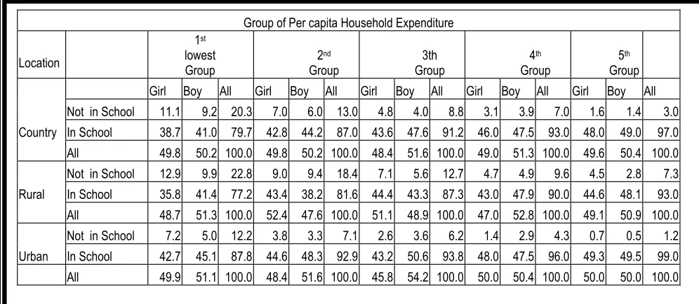
Table 6 illustrates the percentage of children in school and children not in school divided into expenditure per capita group and location. Households have been ranked by expenditure per capita and grouped into 5 expenditure groups. On average the children who did not attend school were from poorer families. The proportion of children not in
Figure 1.
The proportion of Children who have Left School, by Gender and Age
0 2 4 6 8 10 12 14
7 8 9 10 11 12 13 14
Age
Pe
rc
e
n
ta
g
e
[image:4.595.105.478.186.441.2]school is higher as we move to lower income groups. Rural areas face higher proportions of children who do not attend school compared to urban areas.
Table 6.
Proportion of Children who Not In School, by Gender, Location and Group of Per Capita Household Expenditure
Source: Author’s calculation based on 1993 IFLS data
b. Model Spesification
Children’s school is a matter of investment for their parents. In the absence of formal old age pension programs, children are expected to support their elderly parents. Potential transfer from children to their elderly parents provides a motive for educational investment at the household level (Maitra and Rammohan, 2001). As we discussed in the previous section Indonesian families expect transfers from their sons in the future (Dursin, 2001). Since there are differences in expected return in education between sons and daughters, for sons being greater than daughters, the gender of a child could reflect proxy expected rate of return of parents. Gender is used as a proxy of parents’ expected rate of return to education, as it may determine which children the parents will get transfers from in the future.
The age of children also affects the decision of whether they will attend school or not, since it may reflect the productivity and physical ability to do certain activities. Older children tend to be involved more in labor market and domestic tasks.
Because we do not have direct information on parental son preference and a direct measure of how much parents care about their children’s education, here we use indirect measures of parental preferences including years of schooling and occupation status of each parent. The parents’ years of schooling and occupations are employed as
Group of Per capita Household Expenditure
Location
1st
lowest Group
2nd
Group
3th Group
4th
Group
5th
Group
Girl Boy All Girl Boy All Girl Boy All Girl Boy All Girl Boy All
Not in School 11.1 9.2 20.3 7.0 6.0 13.0 4.8 4.0 8.8 3.1 3.9 7.0 1.6 1.4 3.0
Country In School 38.7 41.0 79.7 42.8 44.2 87.0 43.6 47.6 91.2 46.0 47.5 93.0 48.0 49.0 97.0
All 49.8 50.2 100.0 49.8 50.2 100.0 48.4 51.6 100.0 49.0 51.3 100.0 49.6 50.4 100.0
Not in School 12.9 9.9 22.8 9.0 9.4 18.4 7.1 5.6 12.7 4.7 4.9 9.6 4.5 2.8 7.3
Rural In School 35.8 41.4 77.2 43.4 38.2 81.6 44.4 43.3 87.3 43.0 47.9 90.0 44.6 48.1 93.0
All 48.7 51.3 100.0 52.4 47.6 100.0 51.1 48.9 100.0 47.0 52.8 100.0 49.1 50.9 100.0
Not in School 7.2 5.0 12.2 3.8 3.3 7.1 2.6 3.6 6.2 1.4 2.9 4.3 0.7 0.5 1.2
Urban In School 42.7 45.1 87.8 44.6 48.3 92.9 43.2 50.6 93.8 48.0 47.5 96.0 49.3 49.5 99.0
indirect measures of how much parents care about their children’s education. The higher the education of parents and the broader their knowledge, the more they tend to have awareness of their children’s education. This study divides parent occupations into two categories – self-employment and otherwise. We may expect that self-employed parents tend to need more help from their children in running their business. As a consequence of this they tend to pay less attention to their children’s education.
Though tuition fees for elementary school have already been abolished, in reality there are various costs related to education, such as uniforms, parent contributions and books. These costs only represent the direct costs. In fact there are other costs that play an important role for parents in their decisions regarding children’s education. In Indonesia, particularly for poor families, children often help their parents either in the labour market or domestic tasks. The presence of grandparents may have an important role in families’ activities. They can be involved in doing domestic tasks, so that they can reduce children’s involvement in doing housework or even totally substitute for them (Liu, 1998). On the other hand, Liu (1998) also mentions that households with children under 5 years old will tend to have higher demand for home production, specifically in the children services area. More children under 5 years old may also demand more child care service from the mother. Because of this older children may have to substitute for their mother in doing some domestic tasks.
Information on school fees and distance or travel time are not available. Nonetheless the survey has information about grandparent presence in the household. Also, the data allow us to calculate the number of children under 5 years old in each household. This information provides remedies for the lack of information on the direct costs of education, distance or travel time and indirect or opportunity costs. This study use a dummy for presence of grandparents and number of children under age 5 years in the household as proxies for cost of schooling in terms of home production and children’s time forgone.
Income is likely to be a key household characteristic in determining the demand for children’s education, since obviously income is an important constraint for households. To capture the resource constraint parents face in making investment decisions, we use household expenditure instead of income. There are two reasons for this. First, total household expenditure is easier to measure than total household income, and it is measured with less error of measurement. Second, income may be subject to transitory fluctuation since savings tend to smooth expenditure over time (Tansel, 1998). Initially this paper attempted to employ a direct measure of yearly household income, but the results were not satisfactory. Ultimately monthly household expenditure is used.
usually used to capture quality of school such as: number of textbook per student, teacher-pupil ratio, class room-student ratio, number of trained teacher (Dreze and Kingdon, 2000; Colclough et al, 2000; Liu, 2001, Handa, 2002). Teacher-pupil ratio and dummy of library resources are employed as schools quality indicators in this paper.
Some other household characteristics such as rural – urban (whether a household is located in rural or urban areas), Java, Sumatra, Bali, Kalimantan, NTB (whether household is located in java, Sumatra, Bali, Kalimantan or NTB) are employed as control variables.
Because the data are dichotomous (that is, the child is either in school or not), the probit model is appropriate1.
Assume we have a regression model like the following:
β
β
ε
i ij j k j iX
y
=
+
Σ
+
=1
0
*
(1)Where yi = 1 if yi* > 0
0 if otherwise (2) yi* is unobservable variable or “ latent” variable and ε is the residual
Assume var (ε) = 1 from (1) and (2) we get
Pi = Prob (yi = 1) = Prob
[
(
)]
1
0 j ij
k
j
i
β
β
X
ε
=Σ
+
−
>
= 1 – F [-(β0 + Σβj Xij)] (3)
Where F is the cumulative distribution function ε. If the distribution of ε is symmetric , we can rewrite equation (3) as:
Pi =
(
)
1
0 j ij
n
j
X
F
β
β
=
Σ
+
Since 1 – F(- Z) = F (Z), then the maximum likelihood function can be written as:
L =
∏
∏
= =
−
0 1)
1
(
i i y i y jP
P
In the case F (Z) =
)
exp(
1
)
exp(
i iZ
Z
+
, taking log of the two sides we get:Log
)
(
1
)
(
i iZ
F
Z
F
+
= ZiProb (yi) = β0 + βi1 X + βi2 Y + βi3 W + βi4 Z + Ui
Where, yi = 1 if the child is in school
0 if otherwise
1
X = Children’s characteristics
Y = Parental characteristics W = Household characteristics Z = Community variables
Referring to the previous discussion, the dependent variables can be pooled together into these following three main groups. The first group is children’s characteristics, including age, squared term of age and gender. The second group is parental characteristics consisting of parent’s year of schooling and dummies for occupations. The third group is household characteristics including monthly household expenditure, number of children under 5 year old in the household, the presence of grand parents and a dummy for urban-rural and location (island). The last group is community variables such as teacher-pupil ratio and library resources that also capture the quality of education. The model allows the relationship between being in school and age to be non-linear.
[image:8.595.79.526.473.771.2]C. Estimation Results
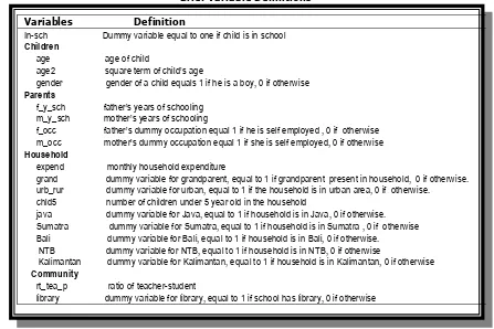
Table 9 displays the variable definitions and Table 10 presents the marginal probit estimates, the probit regression coefficients and t values for the regressions where the dependent variable is a dichotomous indicator of whether or not a particular child was attending school at the time of the survey.
[image:8.595.78.528.491.772.2]The Chi-square statistic rejects the null hypothesis that all the estimated coefficients are jointly equal to zero. The Pseudo R-squared indicates the model is reasonably good.
Table 7.
Brief Variable Definitions
Variables Definition
In-sch Dummy variable equal to one if child is in school
Children
age age of child
age2 square term of child’s age
gender gender of a child equals 1 if he is a boy, 0 if otherwise
Parents
f_y_sch father’s years of schooling m_y_sch mother’s years of schooling
f_occ father’s dummy occupation equal 1 if he is self employed , 0 if otherwise m_occ mother’s dummy occupation equal 1 if she is self employed, 0 if otherwise
Household
expend monthly household expenditure
grand dummy variable for grandparent, equal to 1 if grandparent present in household, 0 if otherwise. urb_rur dummy variable for urban, equal to 1 if the household is in urban area, 0 if otherwise.
chld5 number of children under 5 year old in the household
java dummy variable for Java, equal to 1 if household is in Java, 0 if otherwise.
Sumatra dummy variable for Sumatra, equal to 1 if household is in Sumatra , 0 if otherwise Bali dummy variable for Bali, equal to 1 if household is in Bali, 0 if otherwise.
NTB dummy variable for NTB, equal to 1 if household is in NTB, 0 if otherwise
Kalimantan dummy variable for Kalimantan, equal to 1 if household is in Kalimantan, 0 if otherwise
Community
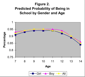
To assess the implications of the estimated model, we calculate the predicted
probabilities of being in school for both boys and girls. The model allows the relationship between being in school and age to be non-linear. We find that both linear and quadratic
terms are statistically significant. The marginal probit result presented in Table 10
suggests that children in schooling increases at a diminishing rate with the age of the
child. There is a positive relationship between the probability of being in school and
children’s age. The increase in the age of child is associated with a significant increase in
the probability of school attendance. This unusual case is also found by Duraisamy
(2000) in India, Maitra and Rammohan (2001) in South Africa, Fitzsimons (2002) in Indonesia, and Gibson (2002) in Papua New Guinea. In their paper Maitra and
Rammohan (2001) demonstrate that when they use data of children between 7 to 24
years old, they find that the age of the child has a negative relationship with the
probability of being in school. However, when they subdivide the sample into different
age categories, they find that age effect is not the same for the different age categories.
In the age group 7 to 12 there is a positive effect of age to probability of being in school.
For children in the age groups 13 to 17 and 18 to 24 the effect is negative. In other words the age effects on the probability of being in school vary over the age range. For
the younger age group, the effect of age tends to be positive, while for the older age
group the effect tends to be negative. This is because as children grow older,
employment opportunities increase and so do alternative activities at home, thus the
opportunity costs of education increase. The results from previous studies above may
provide explanations of why in our study, we have positive effects of age on probability
of being in school. This is because we employ children with the age 7 to 14 categorized in younger age group.
The probit estimation indicates significant gender differences in children’s
schooling behaviour. The probability of girls being in school is one percent lower than
that of boys.
Parental characteristics affect the children’s schooling behaviour. The results
confirm that for the probabilities of being in school, both father and mother’s education
matter. Interestingly, the empirical result in this paper suggests that the mother’ education has a slightly stronger positive effect than fathers’. This may because mothers
spend more time in home investment than do fathers. One more year of schooling of
more year schooling of fathers it increases only 0.7%. This implies that mothers’
education is an important factor in affecting child school attendance. Separate estimation
of girls’ and boys’ school participation outcomes indicate that mothers’ education is more
important for girls, while fathers’ education is more important for boys. One more year of schooling of fathers increases the probability of being in school by 0.8% for boys and
only 0.5% for girls. On the other hand one more year of schooling of mother increases
the probability of school attendance by 1.2% for girl and only 0.6% for boy. This result
shows how important is the effect of girls’ schooling, since girls’ education has a trickle
down effect on the next generation. The higher the mothers’ education the more
attention they pay to their children’s schooling and as a result, their children, especially
girls, may be expected get a better education and this expands education in the next
generation.
Turning to the household characteristics, we find that income effect captured
through the household income (proxied by household expenditure) variable is positive
and significant. But the magnitude is small. Children belong to richer household have a
higher probability of being enrolled in school. An increase in the household income by Rp
10,000 (roughly US$5) will increase children’s probability of school participation by
0.028%. Interestingly, for a separate probit regression, household income is significantly
positive only for girls. An increase the household income by Rp 10,000 will increase girls’ probability of school attendance by 0.08%. This implies that girls’ chance of going to
school is more sensitive to household income; therefore education is categorized as a
luxury good for girls. The household income only matters for girls, which may imply that
the parental preference for sons factor and cultural values have a stronger role in
educating boys than resources available to the household, but the magnitude is not
large.
Further, the negative effect of number of children under five years old is significant for girls. This confirms that for the girls there is trade off between attending
school and substituting for the mother in doing domestic tasks as well as taking care of
younger children. The result show that one more child under 5 year decreases the
probability of girls between 7 to 14 year of age attending school by 1.2 percentage
Table 8.
Estimated Probit Result for the Gender Differences in Education
Variable Girl Boy All
Coef. dF/dx t-value Coef. dF/dx t-value Coef. dF/dx t-value
Children’s characteristics Gender
Age Age2
Parental characteristics Father’s year of schooling Mother’s year of schooling Father’s occupation dummy Mother’s occupation dummy Household characteristics
Monthly household expenditure Grandparent
Children under 5 Rural – urban Java Sumatra Bali NTB Kalimantan Community variable Teacher-pupil ratio Library Constant 0.617 -0.032 0.033 0.086 -0.080 -0.056 5.88e-07 0.015 -0.085 0.139 0.224 0.205 0.232 0.128 -0.303 4.559 -0.051 -2.445 0.085 -0.004 0.005 0.012 -0.011 -0.008 8.08e-08 0.002 -0.012 0.019 0.031 0.026 0.027 0.016 -0.051 0.627 -0.007 3.48*** -3.81*** 2.31** 5.20*** -0.84 -0.67 3.30*** 0.08 -1.72* 1.51 1.46 1.26 1.03 0.66 -1.31 1.69* -0.47 0.692 -0.035 0.057 0.045 0.006 0.049 8.17e-07 0.111 -0.041 0.178 0.253 0.480 0.334 0.021 0.070 0.596 0.106 -2.761 0.094 -0.005 0.008 0.006 0.0008 0.007 1.11e-08 0.014 -0.006 0.024 0.035 0.055 0.036 0.003 0.009 0.081 0.015 3.79*** -4.16*** 4.14*** 2.75*** 0.06 0.55 0.96 0.62 -0.79 1.97** 1.66 2.86*** 1.50 0.11 0.31 0.22 0.94 0.093 0.647 -0.033 0.047 0.065 -0.029 -0.002 2.00e-07 0.058 -0.064 0.173 0.251 0.336 0.303 0.087 -0.107 2.536 0.026 -2.613 0.013 0.091 -0.005 0.007 0.009 -0.004 -0.0003 2.82e-08 0.008 -0.009 0.024 0.036 0.042 0.035 0.011 -0.016 0.357 0.004 1.70* 5.11*** -5.61*** 4.85*** 5.66*** -0.43 -0.04 2.66*** 0.47 -1.82* 2.71*** 2.34** 2.91*** 1.93** 0.64 -0.67 1.34 0.34 Number of observations
Chi-square (degree of freedom) Pseudo R-square 2166 208.51 (17) 0.1375 2235 155.70 (17) 0.1100 4401 346.58(18) 0.1181 Notes: a). dF/dx is for discrete change of dummy variable from 0 to 1.
b). *** = significant at the 1% level ** = significant at the 5% level * = significant at the 10% level
Figure 2.
Predicted Probability of Being in
School by Gender and Age
0.75 0.8 0.85 0.9 0.95 1
7 8 9 10 11 12 13 14
Age
Percen
ta
g
e
The effect of an urban location is statistically significant when we regress boys and girls all together. The marginal effect shows that holding all other explanatory variables at their sample means, urban children have 2.4 percentage points higher probability of being enrolled in school than rural children. When we estimate the equation for boy and girl separately, the dummy urban variable is significant only for boys. Boys in urban areas have 2.4% higher probability of being in school compared to boys in rural areas.
The effect of geographical location namely Java, Sumatra and Bali are also significant. It means children living on these island are more likely to be enrolled. This is not surprising because these three areas, especially Java, are relatively better developed compared to Sulawesi.
On the supply side of schooling, we find that teacher-pupil ratio has a positive significant effect only for girls. School quality is an important factor for girls in deciding whether they will be sent to school or not. For boys there is no effect from school quality, they will be sent to school no matter if the school quality is good or not.
[image:12.595.160.500.439.748.2]Figure 2 demonstrates the predicted probability of children of being in school. From the age 7 to 11 generally the predicted probability of being in school is between 0.92% to 0.95%. Children’s predicted probability of being in school decreases when they grow older. The older the children the lower their predicted probabilities of being in school. From age 11 the probability of being in school starts to decline. For all age categories (7 to 14) the predicted probability of being in school for girls is always lower than for boys.
D. Concluding Remarks
Nationally representative household survey data have been used in this paper to examine the factors affecting the school enrolment and the nature of gender differences in school enrolment among 7 to 14 year old boys and girls in Indonesia. The results obtained from the study confirm that gender differences are important in determining the likelihood of children being in school. In terms of predicted probability of attending school, our estimates suggest that generally girls have lower probability of going to school compared to boys.
Our results also suggest that family background variables such as parental schooling and income have a positive effect on children’s school attendant. Paternal and maternal education significantly affects enrolment of boys and girls but in different manner. While fathers’ education is more favourable affect boys’ schooling, mothers’ education is more essential for girls’ schooling.
Also household income has a positive effect on children’ schooling. Girls are more sensitive to the constraint on available resources. The likelihood of girls being in school is also influenced by the number of children under 5 years old in the household. The more children under 5 years old in the household the less likely it is for a girl to be in school.
Regional differences and urban area are found to be important in affecting children’s participation in school. Urban children are more likely to be in school than rural children. Children from Java, Sumatra and Bali have a higher probability of attending school. This may be because these islands are relatively more developed than Sulawesi.
quality improvement need to be implemented. These include improving school facilities and school building quality, providing textbooks, and improving teachers’ skill and quality by giving special training and short courses.
References
Ablett, J., and Slengesol, I.A.(2000). “Education in Crisis The impact and Lessons of the East Asian Financial Shock, 1997-99,” Education for All 2000, Thematic Study, World Bank, Human Development Network.
Ahmed, J., Angeli, A., Biru, A., and Salvini, S. (2001). “Gender Issues, Population and Development in Ethiopia,” Central Statistical Authority, Addis Ababa, Ethiopia., and Institute for Population Research, National Research Council, Rome, Italy.
Alisjahbana, S. Armida. (1998). Demand for Children’s Schooling In Indonesia: Intrahousehold Allocation of Resources, The Roles of Prices and Schooling
Quality, Department of Economics and Development Studies, Padjadjaran
University, Bandung. (mimeo)
Becker, G.S., and Tomes, N. (1976). “Child Endowments and the Quantity and Quality of Children,” Journal of Political Economy, Vol. 84, pp. s43-s162.
BPS. (1997). Statistik Indonesia: statistical pocketbook of Indonesia, Jakarta
Colclough, C., Rose, P., Tembon, M. (2000). “Gender Inequalities in Primary Schooling: The Roles of Poverty and Adverse Cultural Practice,” IDS working paper 78
Deolalikar, B. Anil. (1993). “Gender Differences in The Returns to Schooling and In School Enrollment Rates in Indonesia,” The Journal of Human Resources, Vol. 28, isuue 4, pp.899-932.
Dreze, J., and Kingdon, G.G. (2000). School Participation in Rural India, Centre for Development Economics, Delhi School of Economics, Delhi and The University of Oxford.
Duflo, E. (2000). “Schooling and Labor Market Consequences of School Construction in Indonesia: Evidence from an Unusual Policy Experiment,” Working paper 7860,
http://www.nber.org/papers/w7860.
Duraisamy, M. (2000). “Child Schooling and Child Working in India,” Paper presented in the Eight World Congress of The Econometric Society at University of Washington, Seatle WA, August 11-16 2000.
Dursin, R. (2001). “Indonesia: Education Still a Male Domain,” Asia Times Online,
Fitzsimons, E. (2002). Risk, Education and Child Labour in Indonesia, University College London and Institute For Fiscal Studies, London.
Gertler, P., Levine, I.D., and Ames, M. (2002). Schooling and Parental Death, University of California, Berkeley.
Gibson, J. (2002). Who’s not in School? Economic Barriers to Universal Primary Education
in Papua New Guinea, Department of Economics University of Waikato.
Handa, S. (2002). “Raising Primary School Enrolment in Developing Countries The Relative Importance of Supply and Demand,” Journal of Development Economics, 69, pp. 103-128.
Hanmer, L., and Naschold, F. (2000). “Attaining the International Development Targets: Will Growth be enough?” Development Policy Review, 8, pp 11-36.
Hartono, D., and Ehrman, D. (2001). “The Indonesian Economic Crisis and Its Impact on Education Enrolment and Quality,” Paper presented at Seminar organized by the Institute of Southeast Asian Studies, 23rd March 2001, Singapore.
Insukindro. (No Date). Kemiskinan dan Distribusi Pendapatan di Daerah Istimewa
Yogyakarta 1984 – 1987, Fakultas Ekonomi Universitas Gadjah Mada,
Yogyakarta.
Kambhampati, S. Uma, and Pal S. (2000). “School Participation Among Boys and Girls in Rural India: Role of Household Income and Parental Bargaining,” Paper presented at the Royal Economic Society, London.
Kevane, M., and Levine, D. (2000). “The Changing Status of Daughters in Indonesia,” Paper presented at Seminars at U.C. Berkeley and U.C. Riverside.
Knowles, C. James. (1999). “The Social Crisis in Asia,” Paper presented at twelfth workshop on Asian Economic Outlook, 23 Nov 1999, ADB.
Liu, Y.C. (1998). “Economics of Time Allocation of Children in Vietnam,” Phd dissertation at Australian National University, Unpublished.
Liu, Y.C. Amy. (2001). “Flying Ducks? Girls’ Schooling in Rural Vietnam,” Asian Economic
Journal, Vol. 15, No. 4, pp. 385-403.
Maddala, G.S. (1992). Inroduction to Econometrics, (second edition), Macmillan publishing company.
Maitra, P. and Rammohan, A. (2001). “Schooling and Educational Attainment of Shout Africa Children,” Revised versions of University of Sydney working paper no 99-04.
Training Center at Brown University and The Society of Labor Economists Internet Seminar Series.
Millimet, L. Daniel. (2003). Quantity versus Quality Revisited: The Effect of Household
Size on Schooling in Indonesia, Southern Methodist University.
Mincer, J. (1974). Schooling Experience and Earnings, New York: Columbia University Press.
Oxaal, Z. (1997). “Education and Poverty: A Gender Analysis,” Report prepared for the Gender Equality Unit, Swedish International Development Corporation Agency (SIDU), Institute of Development Studies, University of Sussex, Brighton.
Pal, S. (2002). How Much of The Gender Differences in Child School Enrollment can Be
Explained: Evidence from Rural India, Economics Section, Cardiff Business
School, Curdif University, (mimeo)
---. (2003). How Much of The Gender Differences in Child School Enrollment can Be
Explained: Further Evidence from Rural India, Economics Section, Cardiff
Business School, Curdif University, (mimeo)
Parish, L. William, and Willis, J.R. (1993). “Daughter, Education, and Family Budgets: Taiwan Experiences,” The Journal of Human Resources, vol. 28, issues 4, Special issue: Symposium on Investment in Women’s Human Capital and Development, pp. 863-898.
Pasqua, S. (2001). “A Bargaining Model for Gender Bias in Education in Poor Countries,” Working Paper, Centre for Household, Income, Labour and Demographic Economics, University di Torino, Torino, Italy.
Pitt, M., and Rosenzweig, M.R. (1990). Estimating the Intrafamily Incidence of
Households, University of Minnesota.
Quisumbing, R. Agnes, and Maluccio, A.J. (1999). “Intrahoushold Allocation and Gender Relations: New Empirical Evidence,” Policy Research Report on Gender and Development, working paper series, No. 2, The World Bank, Development Research Group, Poverty Reduction and Economic Management Network.
Ray, R. (2001). The Determinat of Child Labour and Child Schooling in Ghana, School of Economics, University of Tasmania.
Satrividina, R.(1997). “Determinants and Consequences of Early Marriage in Java, Indonesia,” Asia Pasific Population Journal, Vol. 12, No. 2,
http://www.unescap.org/pop/journal/1997/v12n2a2.htm.
Tansel, A. (1997). “Schooling Attainment, Parental Education, and Gender in Cote d’Ivoire and Ghana,” Economic Development and Cultural Change, 45, pp: 825-56
---. (1998). “Determinants of School Attainment of Boys and Girls in Turkey,” Center Discussion paper no. 789, Economic Growth Center, Yale University.
Unicef. (2003). “Girls’ Education in Indonesia, http://www.unicef.org/programme
/girlseducation/action/ed-profiles/indonesiafinal.pdf..
University of Manchester. (1998). “Volume 3: Country Profiles of Investment Opportunities in Private Education in Developing Countries,” Report to The International Finance Corporation.
World Bank. (2002). “Indonesia Country Brief,” http://Inweb18.worldbank.org
/eap/eap.nsf/680c532d463b70a852.
---.(2003).“Edstat-Thematic Data: Indonesia,” http://devdata.worldbank.org
/edstats/thematicDataonEducation/Ge.