EVALUATION OF THE VRP COMPLETION WITH
DEVELOPING HYBRID GENETIC ALGORITHM
USING FUZZY LOGIC CONTROLLER MODEL
Yogi Yogaswara1
1 Industrial Engineering Department, Pasundan University
Jl. Dr. Setiabudhi 193 Bandung, Indonesia
E-mail: [email protected]
ABSTRACT
This study discusses the results of modified Vehicle Routing Problem calculation using Hybrid Genetic Algorithm (HGA). It is shown that by modifying the Genetic Algorithm can provide good and effective solution. The results obtained were compared with the Standard Genetic Algorithm (SGA) and Modified Genetic Algorithm (MGA) to various problems the size of the node. For medium number of nodes (scenario 2) MGA get good results, but the resulting solution in the case of a small number of nodes that actually leads to local optima. However, it can be determined that the HGA is better than SGA and MGA. It could be argued that all three models of the genetic algorithm is an effective algorithm, if used in the right conditions.
Key words: Node, VRP, SGA, MGA, HGA, FLC Model,
1. INTRODUCTION
Increasing the efficiency of the transportation system can be done to maximize the utility of existing transportation. To reduce transport costs and to improve service to customers, is necessary to find the best path or route of transportation, which can minimize the distance and time, without prejudice to the vehicle carrying capacity. Problems which aims to create an optimal route, for a group of vehicles, in order to serve a number of customers referred to as the problem Vehicle Routing Problem (VRP).
The Genetic Algorithm has the ability to do global search a wider compared with other meta-heuristic algorithms and is one that is flexible, so it can be applied to various types of problems as well as in combination with other methods (hybrid). In the VRP problems, including the development of the algorithm is to modify the number of steps on a genetic algorithm, or by combining it with local search or other methods for meta-heuristics can produce better performance. One application is a hybrid between genetic algorithm to determine the value of the parameters that can provide an optimal solution, by combining (hybrid) genetic algorithm with fuzzy logic controller to
perform automatic fine-tuning of the genetic algorithm parameter values so hopefully obtain more results close to optimal.
Fuzzy logic provides a simple way to illustrate the definitive conclusions from the information that is ambiguous, vagues, or inaccurate. Fuzzy logic offers some unique characteristics that make it a good choice for many control problems. These characteristics include the concept is easy to understand, very flexible, can tolerate less precise data, and be able to model complex nonlinear functions.
2. FORMULATION MODEL
This study focused on modeling VRP and their modifications into the GA method consisting of the standard genetic algorithm, modified genetic algorithm and hybrid genetic algorithm using fuzzy logic controller. From the results of this study can be known which of the three types of methods that can produce the best solution, both from the acquisition of an optimal solution and time calculations.
2.1. Model Assumptions
a. Single depot problem
b. Shortest distance problems with the track conditions and vehicle capacity are considered equal.
c. Time windows are not considered
d. Crossover probability value used is 0.65 (the value used generally ranged from in the current and next generation using fuzzy decision table.
g. Initial population of randomly generated h. The number of generations was made 10
times for each method i. Split delivery is not allowed.
j. All the line are considered 2-way, always available, and congestion or technical barriers are ignored
k. Vehicles are considered similar (homogenous).
l. All costs are considered fixed
m. distance of node i to node j = distance of node j to node i.
n. Deterministic Demand and fixed at each visit
o. Range of Cooling Ratio (μ) is between 0 and 1. In this study the value of cooling ratio used was 0.999.
p. Initial Different degree is assumed 0.6
2.2. VRP procedures with Fuzzy Logic
5. The establishment of new population 6. Determine the GA parameter values for
the next iteration by using Fuzzy Logic Controller (FLC)
7. Termination Test
8. Determine the best solution
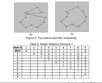
2.3. The 2-opt Algorithm and Smoothing Method
a. The 2-opt Algorithm.
A good tour is if there is no cross in it. The principle of this method is to remove the two trajectories intersect, and outlines the tour into two paths in another way such that no city, check whether there's a cross between a track formed of the city "a" to the city "b" where, "b" is the city that comes after "a" to any track. Parameters are crossing a tour can be described as follows: we let the city "a" is the currently selected city, next(a) is the city came after a city tour in the sequence. And if "b" any different city of the city "a" and the next(a). The tour can now be fixed with the following conditions:
d(a, next(a)) + d(b, next(b)) > d(next(a), next(b)) + d(a,b).
Furthermore, a new arc is (next (a), next (b) and (a, b) as shown in Figure 1.
Figure 1. Elimination of intersection with the 2-opt algorithm
b. Smoothing Algorithm
description of the smoothing algorithm is as follows:
Step 1:
Make a list of the nearest city pair (near list) for each city
Step 2:
Checks for each city on the tour is going sharpness. The sharpness parameter can be formulated as follows: for example, the distance d (i, j) represents the distance from city i to j. And also, if the city "a" is a city that is being checked, "b" is the city closest to the "a" and "c" is a neighbor with a "b" too close to "a". Parameter presence of sharpness in the tour are the following conditions:
d( prev(a),a) + d(a,next(a)) + d(b,d) > d(b,a) + d(a,c) + d( prev(a),next(a))
where, prev (a) and next (a) is the town before and after the city "a" in the tour sequence.
Step 3.
If the condition in step 2 is met, do smoothing by changing the trajectory of the tour. If the trajectory of L (prev (a), a), L (a, next (a)), L (b, a) is a trajectory that is formed from the city that is being executed. Change the path so that it becomes L (b, a), L (a, c) and L (prev (a), next (a)). Result of
smoothing algorithm can be seen in Figure 2.
3. MODEL IMPLEMENTATION
Genetic algorithm is a heuristic and evolutionary improvement, then the solution is necessary initialization, in case this is a form of VRP initial population as a place to start the search for solutions. The composition of random numbers represent the order of the route taken by a vehicle which then calculated the fitness of each chromosome. In this study the application of the model performed on two scenarios, and three models of genetic algorithms. So that each scenario and model of genetic algorithm requires a different population initialization.
3.1. Data Collection
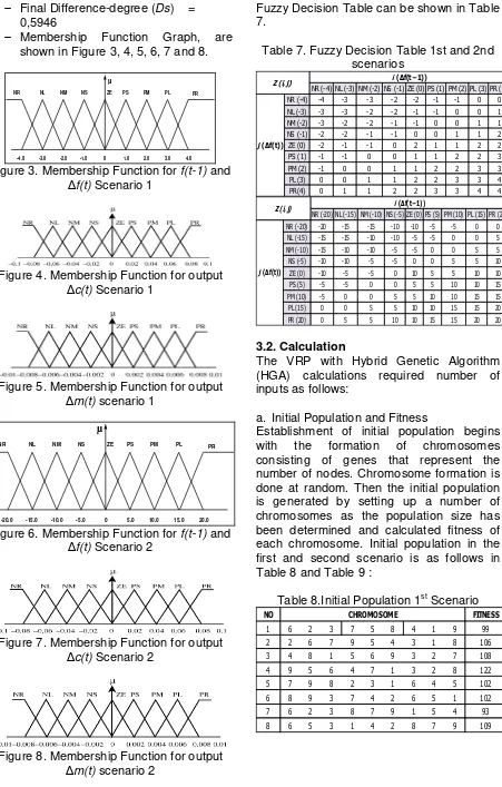
a. The distance between the depot and nodes
Matrix distance between the depot and nodes as well as node and the nodes on the complete 1st scenario can be seen in Table 3
and Table 4 for 2nd scenario.
Figure 2. Tour before and after smoothing
Table 3. Nodes Distance Scenario 1
FROM/TO 1 2 3 4 5 6 7 8 9
DEPOT 14 7 13 12 5 2 7 9 10
1 - 15 15 16 6 12 12 15 7
2 - 6 11 9 3 7 10 12
3 - 11 9 7 7 10 12
4 - 10 8 8 4 23
5 - 6 6 9 13
6 - 4 7 9
7 - 7 5
8 - 12
-Table 4. Nodes Distance Scenario 2
b. Demand for Each Nodes
Data demand at each node randomly generated from 20 to 55 units for scenario 1, and from 2 to 18 units for problems in scenario 2. Data demand shown in Table 5.
Table 5. Scenario 1 and 2 Data Demand
NODE DEMAND
In this study the type of vehicle used in each scenario are assumed similar (homogeneous) with the number of vehicles available is unlimited. However, to obtain the best solution, the number of vehicles used is
minimum. Given the capacity of the vehicle in scenario 1 is at 140 units and the capacity of the vehicle in scenario 2 is for 60 units. The cost for both scenarios is the same and consists of fixed costs and variable costs that have assumed Rp per km.
d. Genetic Operator Parameters
Genetic Operator Parameters obtained by random or refer to the related literature. The parameters are as follows in Table 6.
Table 6. Genetic Operator Parameters for each Scenarios
Auxillary data consists of parameters which are used to support the Modified Genetic Algorithm (MGA) and a Hybrid Genetic Algorithm (HGA) model calculation, are :
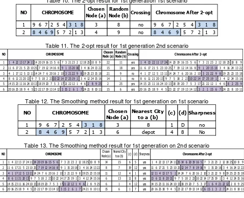
Final Difference-degree (Ds) = 0,5946
Membership Function Graph, are shown in Figure 3, 4, 5, 6, 7 and 8.
1.0 2.0 3.0 4.0
-1.0 -2.0 -3.0
-4.0 0
NR NL NM NS ZE PS PM PL PR
µ
Figure 3. Membership Function for f(t-1) and Δf(t) Scenario 1
Figure 4. Membership Function for output Δc(t) Scenario 1
Figure 5. Membership Function for output Δm(t) scenario 1
5.0 10.0 15.0 20.0 -5.0
-10.0 -15.0
-20.0 0
NR NL NM NS ZE PS PM PL PR µ
Figure 6. Membership Function for f(t-1) and Δf(t) Scenario 2
Figure 7. Membership Function for output Δc(t) Scenario 2
Figure 8. Membership Function for output Δm(t) scenario 2
Fuzzy Decision Table can be shown in Table 7.
Table 7. Fuzzy Decision Table 1st and 2nd scenarios
NR (-4) NL (-3) NM (-2) NS (-1) ZE (0) PS (1) PM (2) PL (3) PR (4)
NR (-4) -4 -3 -3 -2 -2 -1 -1 0 0
NL (-3) -3 -3 -2 -2 -1 -1 0 0 1
NM (-2) -3 -2 -2 -1 -1 0 0 1 1
NS (-1) -2 -2 -1 -1 0 0 1 1 2
ZE (0) -2 -1 -1 0 2 1 1 2 2
PS (1) -1 -1 0 0 1 1 2 2 3
PM (2) -1 0 0 1 1 2 2 3 3
PL (3) 0 0 1 1 2 2 3 3 4
PR(4) 0 1 1 2 2 3 3 4 4
Z (i, j) i (Δf(t−1))
j (Δf(t))
NR (-20) NL (-15) NM (-10) NS (-5) ZE (0) PS (5) PM (10) PL (15) PR (20) NR (-20) -20 -15 -15 -10 -10 -5 -5 0 0 NL (-15) -15 -15 -10 -10 -5 -5 0 0 5 NM (-10) -15 -10 -10 -5 -5 0 0 5 5 NS (-5) -10 -10 -5 -5 0 0 5 5 10 ZE (0) -10 -5 -5 0 10 5 5 10 10 PS (5) -5 -5 0 0 5 5 10 10 15 PM (10) -5 0 0 5 5 10 10 15 15 PL (15) 0 0 5 5 10 10 15 15 20 PR (20) 0 5 5 10 10 15 15 20 20 Z (i, j) i (Δf(t−1))
j (Δf(t))
3.2. Calculation
The VRP with Hybrid Genetic Algorithm (HGA) calculations required number of inputs as follows:
a. Initial Population and Fitness
Establishment of initial population begins with the formation of chromosomes consisting of genes that represent the number of nodes. Chromosome formation is done at random. Then the initial population is generated by setting up a number of chromosomes as the population size has been determined and calculated fitness of each chromosome. Initial population in the first and second scenario is as follows in Table 8 and Table 9 :
Table 8.Initial Population 1st Scenario
NO FITNESS
1 6 2 3 7 5 8 4 1 9 99
2 2 6 7 9 5 4 3 1 8 106
3 4 8 1 5 6 9 3 2 7 108
4 9 5 6 4 7 1 3 2 8 122
5 7 9 8 2 3 1 6 4 5 102
6 8 9 3 7 4 2 6 5 1 102
7 6 2 3 8 7 9 1 5 4 93
8 6 5 3 1 4 2 8 7 9 109
Table 9.Initial Population 2nd Scenario
1 1 4 22 13 17 24 10 25 7 19 12 14 5 6 20 3 21 23 8 16 18 15 11 2 9 383 2 10 6 17 21 5 23 11 14 20 9 16 15 22 8 19 1 25 7 18 3 4 12 24 13 16 374 3 14 15 23 18 7 17 20 13 16 19 9 2 5 3 24 8 22 12 1 4 6 21 25 10 11 328 4 13 16 24 15 9 4 1 10 7 19 12 11 22 3 6 21 23 14 25 5 20 8 18 2 17 371 5 4 17 1 15 20 13 9 7 24 14 6 5 16 2 10 3 12 22 11 8 19 25 23 21 18 282 6 15 3 24 19 8 1 5 21 13 16 23 10 11 18 7 22 25 17 20 4 12 2 6 14 9 338 7 14 9 3 12 7 17 4 6 24 15 22 2 13 11 25 18 23 19 1 5 10 20 8 21 16 371 8 14 15 23 25 16 24 9 13 2 19 20 7 5 3 17 8 22 12 1 4 6 21 18 10 11 327 9 8 6 17 21 5 15 11 14 20 18 2 23 10 22 7 1 25 19 9 3 4 12 24 13 16 360 10 19 4 21 18 7 17 20 25 16 2 6 13 3 5 9 24 8 23 15 10 1 11 22 14 12 375 11 14 9 25 11 7 17 4 19 24 18 22 2 13 12 3 15 21 6 1 5 10 20 8 23 16 361 12 20 16 11 18 10 7 5 23 22 17 19 13 14 12 3 15 21 6 1 4 24 2 8 9 25 369
NO CHROMOSOME FITNESS
b. Crossover
Crossover process using Partially Mapped Crossover (PMX) with crossover probability is 0.65.
c. Mutation
This process first randomly select a gene to be mutated. The method used is a Reciprocal Exchange Mutation, in which the
mutation is done by exchanging the value of the two genes at random positions
d. Apply 2-opt method and the smoothing method of the offspring.
This step is a procedure to repair a tour on chromosome contained two populations awal terdapat tour improvement techniques (local search) are used. The first is to adopt the 2-opt improvement methods to eliminate the intersected arc. Further smoothing method is used to eliminate sharpness in order to obtain optimal results. For the case of VRP in this study, to avoid the black hole and get stuck in local optima, then repairing the tour is done only on one route only in one chromosome, so for the exchange of genes is only valid on the route (sub-cromosom) selected only. Determination of sub-chromosome is randomly selected, and sub-chromosome calculated based on the rules of the vehicle capacity.
Table 10. The 2-opt result for 1st generation 1st scenario
1 9 6 7 2 5 4 3 1 8 3 8 no 9 6 7 2 5 4 3 1 8
2 8 4 6 9 5 7 2 1 3 4 9 no 8 4 6 9 5 7 2 1 3
NO CHROMOSOME Chosen Node (a)
Random
Node (b) Crossing Chromosome After 2-opt
Table 11. The 2-opt result for 1st generation 2nd scenario
1 1 4 22 13 17 24 11 14 20 19 16 15 5 6 7 3 21 23 2 12 18 25 10 8 9 22 11 yes 1 4 13 22 11 17 24 14 20 19 16 15 5 6 7 3 21 23 2 12 18 25 10 8 9 2 11 6 17 21 5 23 10 25 7 19 12 14 16 8 9 1 15 20 18 3 4 16 24 13 22 15 18 yes 11 6 17 21 5 23 10 25 7 19 12 14 16 8 9 1 20 15 18 3 4 16 24 13 22
3 4 1 17 12 5 13 11 14 24 7 6 20 16 2 10 3 21 22 9 8 19 25 23 15 18 21 9 no 4 1 17 12 5 13 11 14 24 7 6 20 16 2 10 3 21 22 9 8 19 25 23 15 18 4 8 6 11 21 20 13 9 7 5 18 2 23 10 22 14 17 25 19 1 3 4 12 24 15 16 14 1 no 8 6 11 21 20 13 9 7 5 18 2 23 10 22 14 17 25 19 1 3 4 12 24 15 16 5 14 15 23 11 16 24 10 13 18 19 20 7 5 3 17 21 22 12 1 4 6 2 8 9 25 2 25 yes 14 15 23 11 16 24 10 13 18 19 20 7 5 3 17 21 22 12 1 4 6 8 2 25 9
6 20 16 25 18 9 4 5 23 22 17 19 13 14 12 3 15 2 6 1 7 24 21 8 10 11 15 6 yes 20 16 25 18 9 4 5 23 22 17 19 13 14 12 3 2 1 15 6 7 24 21 8 10 11
Chosen Node (a)
Random
Node (b)Crossing Chromosome After 2-opt
NO CHROMOSOME
Table 12. The Smoothing method result for 1st generation on 1st scenario
1 9 6 7 2 5 4 3 1 8 3 8 1 D no
2 8 4 6 9 5 7 2 1 3 6 depot 4 8 No
NO CHROMOSOME Chosen (c) (d)
Node (a)
Nearest City
to a (b) Sharpness
Table 13. The Smoothing method result for 1st generation on 2nd scenario
1 1 4 22 13 17 24 11 14 20 19 16 15 5 6 7 3 21 23 2 12 18 25 10 8 9 14 15 6 5 yes 1 4 22 13 17 24 11 15 14 6 20 19 16 5 7 3 21 23 2 12 18 25 10 8 9 2 11 6 17 21 5 23 10 25 7 19 12 14 16 8 9 1 15 20 18 3 4 16 24 13 22 8 7 19 12 yes 11 6 17 21 5 23 10 25 12 14 7 8 19 16 9 1 15 20 18 3 4 16 24 13 22 3 4 1 17 12 5 13 11 14 24 7 6 20 16 2 10 3 21 22 9 8 19 25 23 15 18 11 12 4 1 yes 12 11 4 13 17 5 1 14 24 7 6 20 16 2 10 3 21 22 9 8 19 25 23 15 18 4 8 6 11 21 20 13 9 7 5 18 2 23 10 22 14 17 25 19 1 3 4 12 24 15 16 6 13 11 8 yes 13 6 11 8 20 21 9 7 5 18 2 23 10 22 14 17 25 19 1 3 4 12 24 15 16 5 14 15 23 11 16 24 10 13 18 19 20 7 5 3 17 21 22 12 1 4 6 2 8 9 25 6 1 4 12 yes 14 15 23 11 16 24 10 13 18 19 20 7 5 3 17 1 6 4 21 22 12 2 8 9 25 6 20 16 25 18 9 4 5 23 22 17 19 13 14 12 3 15 2 6 1 7 24 21 8 10 11 15 6 1 7 yes 20 16 25 18 9 4 5 23 22 17 19 13 14 12 6 15 1 3 2 7 24 21 8 10 11
Chromosome After 2-opt
(c) (d)
NO CHROMOSOME Chosen
Node (a) Nearest City
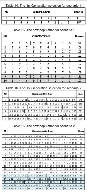
Table 14. The 1st Generation selection for scenario 1
1 9 6 7 2 5 4 3 1 8 111
2 8 4 6 9 5 7 2 1 3 107
NO CHROMOSOME Fitness
Table 15. The new population for scenario 1
1 6 2 3 7 5 8 4 1 9 99
2 2 6 7 9 5 4 3 1 8 106
3 4 8 1 5 6 9 3 2 7 108
4 9 5 6 4 7 1 3 2 8 122
5 7 9 8 2 3 1 6 4 5 102
6 8 9 3 7 4 2 6 5 1 102
7 6 2 3 8 7 9 1 5 4 93
8 6 5 3 1 4 2 8 7 9 109
9 9 6 7 2 5 4 3 1 8 111
10 8 4 6 9 5 7 2 1 3 107
NO CHROMOSOME Fitness
Table 16. The 1st Generation selection for scenario 2
1 1 4 22 13 17 24 11 15 14 6 20 19 16 5 7 3 21 23 2 12 18 25 10 8 9 344 2 11 6 17 21 5 23 10 25 12 14 7 8 19 16 9 1 15 20 18 3 4 16 24 13 22 383 3 12 11 4 13 17 5 1 14 24 7 6 20 16 2 10 3 21 22 9 8 19 25 23 15 18 316 4 13 6 11 8 20 21 9 7 5 18 2 23 10 22 14 17 25 19 1 3 4 12 24 15 16 351 5 14 15 23 11 16 24 10 13 18 19 20 7 5 3 17 1 6 4 21 22 12 2 8 9 25 320 6 20 16 25 18 9 4 5 23 22 17 19 13 14 12 6 15 1 3 2 7 24 21 8 10 11 299
Chromosome After 2-opt
NO Fitness
Table 15. The new population for scenario 2
1 1 4 22 13 17 24 10 25 7 19 12 14 5 6 20 3 21 23 8 16 18 15 11 2 9 383 2 10 6 17 21 5 23 11 14 20 9 16 15 22 8 19 1 25 7 18 3 4 12 24 13 16 374 3 14 15 23 18 7 17 20 13 16 19 9 2 5 3 24 8 22 12 1 4 6 21 25 10 11 328 4 13 16 24 15 9 4 1 10 7 19 12 11 22 3 6 21 23 14 25 5 20 8 18 2 17 371 5 4 17 1 15 20 13 9 7 24 14 6 5 16 2 10 3 12 22 11 8 19 25 23 21 18 282 6 15 3 24 19 8 1 5 21 13 16 23 10 11 18 7 22 25 17 20 4 12 2 6 14 9 338 7 14 9 3 12 7 17 4 6 24 15 22 2 13 11 25 18 23 19 1 5 10 20 8 21 16 371 8 14 15 23 25 16 24 9 13 2 19 20 7 5 3 17 8 22 12 1 4 6 21 18 10 11 327 9 8 6 17 21 5 15 11 14 20 18 2 23 10 22 7 1 25 19 9 3 4 12 24 13 16 360 10 19 4 21 18 7 17 20 25 16 2 6 13 3 5 9 24 8 23 15 10 1 11 22 14 12 375 11 14 9 25 11 7 17 4 19 24 18 22 2 13 12 3 15 21 6 1 5 10 20 8 23 16 361 12 20 16 11 18 10 7 5 23 22 17 19 13 14 12 3 15 21 6 1 4 24 2 8 9 25 369 13 1 4 22 13 17 24 11 15 14 6 20 19 16 5 7 3 21 23 2 12 18 25 10 8 9 344 14 12 11 4 13 17 5 1 14 24 7 6 20 16 2 10 3 21 22 9 8 19 25 23 15 18 316 15 13 6 11 8 20 21 9 7 5 18 2 23 10 22 14 17 25 19 1 3 4 12 24 15 16 351 16 14 15 23 11 16 24 10 13 18 19 20 7 5 3 17 1 6 4 21 22 12 2 8 9 25 320 17 20 16 25 18 9 4 5 23 22 17 19 13 14 12 6 15 1 3 2 7 24 21 8 10 11 299
NO Chromosome After 2-opt Fitness
e. Selection and generating new population The result of selection and generating new population shown at Table 14, 15, 16 and 17.
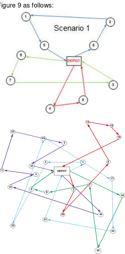
gene sequence 6-3-9-7 | 2-8-4 | 1-5 and 6-2-1 - 5 | 9-7-6-2-1 | 4-8-9 and the total mileage of 91 km which produces 3 route to be taken by the vehicle. Scenario 2 derived chromosome has the best fitness value of chromosome number 23 with the gene sequence 1-4-22-13-17-24-21 | 2-20-6-14-15-16 | 19-10-3 -11-23-12 | 18-25-7-8-9 were divided into 4
Figure 9. The Best Route for Scenario 1 and 2
4. ANALYSIS AND DISCUSSION
HGA model is a model that requires additional parameters required in the procedures of fuzzy logic controller is embedded in the GA models. In use, the
model is quite complex and requires a longer computation time. However, the application of this model gives a very good solution, as shown in scenario 2 model provides the best value compared to the model solution SGA and HGA. Based on the results of the calculation of the scenarios 1 and 2 is also evident that the HGA can provide the best solution that is much faster than the two other models. This is because the autotuning feature derived from the application of Fuzzy Logic Controller (FLC) in this model. FLC will automatically calculate and adjust the probability of crossover and mutation based on the "memory" that have been obtained in previous generations.
Table 16. Final Solution Comparison for Scenario 1
Table 17. Final Solution Comparison for Scenario 2
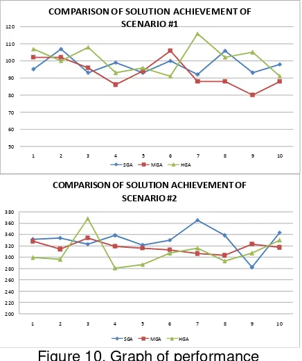
The graphical comparison of performance in obtaining the best solution to the three models used in this study is shown in Figure 10.
Figure 10. Graph of performance comparisons in acquiring the best solution
5. CONCLUSION
The parameters that affect the performance of HGA with FLC determination of which this is the membership function for input and output and a fuzzy decision table. Both were very decisive in changing the crossover probability and mutation probability to be used in the next generation, which will impact on the results of the acquisition of
next generation solutions.
From the results it can be concluded that the model implentasi calculations provide the best solution to the modified models, ie the calculation by using modified genetic algorithm and hybrid genetic algorithm. This suggests that by doing modifications to the genetic algorithm can provide good and effective solution. In problems with node size medium (scenario 2) modified genetic algorithms obtain good results, but the resulting solution in the case of a small number of nodes that actually leads to local optima. However, can not be determined that the hybrid genetic algorithm is better than SGA and MGA. It could be argued that
all three models of genetic algorithm is an effective algorithm, if used in the right conditions.
6. REFERENCES
(a) Auren. (2007). Vehicle Routing Problem. Networking and Emerging Optimization. http://neo.lcc.uma.es/radi-aeb/WebVRP/ (b) Berger, J., Salois, M., (2004, June). A
Hybrid Genetic Algorithm for the Vehicle Routing Problem with Time Windows. Defence R&D Canada, Valcartier, Canada.
(c) Chiang, L.Y. (2002). A Heuristic Approach to Vehicle Routing Problem with Time Window Constraints Based on Hybrid Gentic Algorithm. Unpublished dissertation, Department Of Computer Science, University of Bristol. United Kingdom.
(d) Fisher, M. L. (1994) Optimal solution of Vehicle Routing Problems Using Minimum K-trees, Operations Research, Centre for Computational Intelligence. Germany.
(f) Gen, M., Dan Cheng, R. (1997). Genetic Algoritm and Enginering design. Ashikaga Institute of Technology Ashikaga, Japan, A wiley-Interscience publication, John wiley &Sons, Inc. USA.
(g) Goldberg, D.E (1989). A Comparative Analysis Of Selection Scemes Used In Genetic Algorithm. Department of General Engineering Illinois University. USA.
(h) Goldberg, D.E (1992). Genetic Algoritm in Search,Optimization, and Machine Learning. Addition wesley publishing company,Inc. USA.
(i) Hellmann, M. (2001). Fuzzy Logic Introduction. Laboratoire Antennes Radar Telecom. Rennes Cedex, France. (j) Holland, John, H. (1992, July). Genetic Algorithms. Scientific America. America (k) IDSIA - Istituto Dalle Molle di Studi
sull'Intelligenza Artificiale. (2007).
50
COMPARISON OF SOLUTION ACHIEVEMENT OF SCENARIO #1
COMPARISON OF SOLUTION ACHIEVEMENT OF SCENARIO #2
Vehicle Routing Problem. Http://www.idsia.ch/.
(l) Kovács, Á. (2008, May). Solving the Vehicle Routing Problem with Genetic Algorithm and Simulated Annealing. Unpublished Master Thesis, Computer Engineering. Högskolan Dalarna, Sweden.
(m) Laporte, G. (2002). Classical and Modern Heuristics for the Vehicle Routing Problem. Université de Montréal, Canada.
(n) Rizzoli, A. E., Momtemanni, R., Gambardella, R. M. (2004). Ant Colony Optimisation for vehicle routing problems: from theory to applications. Istituto Dalle Molle di Studi sull’Intelligenza Artificiale. Switzerland. (o) Wang, R., Fukuta, S., Wang, J.H.,
Okazaki, K. (2007, January). A Genetic Algorithm With Conditional Crossover and Mutation Operators and Its Application to Combinational Optimization Problems. Ieice transportation fundamentals, vol. E90-A. Kawasaki, Japan.
(p) Zadeh, A.L. (1988, April). Fuzzy Logic. Univ of california berkeley. California.
AUTHOR BIOGRAPHIES
Yogi Yogaswara is a lecturer in Department