Hybrid Support Vector Regression in Electric Load During National Holiday Season
Rezzy Eko Caraka1,2*, Bens Pardamean2,3#, Sakhinah Abu Bakar1†,Arif Budiarto2‡
1School of Mathematical Sciences, Faculty of Science and Technology
The National University of Malaysia
2Bioinformatics and Data Science Research Center,
Bina Nusantara University, Jakarta, Indonesia, 11480
3Computer Science Department, BINUS Graduate Program – Master of Computer Science
Bina Nusantara University, Jakarta, Indonesia, 11480
Email: *[email protected] [email protected], #[email protected], †[email protected],
Abstract—This paper studies non-parametric time-series approach to electric load in national holiday seasons based on historical hourly data in state electric company of Indonesia consisting of historical data of the Northern Sumatera also South and Central Sumatra electricity load. Given a baseline for forecasting performance, we apply our hybrid models and computation platform with combining parameter of the kernel. To facilitate comparison to results of our analysis, we highlighted the results around MAPE-based and R2-based techniques. In order to get more accurate results, we need to improve, investigate, also develop the appropriate statistical tools. Electric load forecasting is a fundamental aspect of infrastructure development decisions and can reduce the energy usage of the nation.
Keywords—electric load, Support Vector Regression, Hybrid, Kernel, Time Series
I. INTRODUCTION
Electrical system must be developed to fit the increase in electricity needs of customers where the electricity supply should be a priority in its development by the principles of effective and efficient. Therefore, in this case, it is an essential matter for electric service providers [1][2]. Forecasting has a vital role as an absolute requirement that must be done by the service provider company. One of the important things is the
proper electricity forecasting for electricity needs in a particular period. The future prediction will help the solution provider companies to make the right decision. Thus, the planning of electricity operation becomes efficient. Electrical prediction with high precision will attract an imbalance of electrical power between the supply side and the demand side [1].
Forecasting with a huge reason can reduce the imbalance between the side and demand of electricity, will provide the proper foundation for the stability and power of the network to avoid waste of resources in the process of scheduling and to improve. It is essential for the operation of the system as it can provide information that can support and help the system work safely.
With accurate forecasting too, the electricity system will have dynamic stability, quality, and management. Forecasts on electric service providers fall into three categories: short-term forecasting that applies to predictions that occur within a day until the day of up to one week forward. The electric load forecasting is complicated, and it sometimes reveals cyclic changes due to cyclic economic activities or seasonal climate nature, such as the hourly peak in a working day, weekly peak in a business week, and monthly peak in demand planned year [3].
Fig. 1. An Illustration of Electric Load analysis using HYBRID SVR Capture
Analysis
Machine Learning
Feed Forward Neural Network
Generalized Regression Neural Network
Radial Basis
Gaussian Polynomial
Kernel
SVR Traditional
ARIMA
Hybrid SVR Electric
Power Load
Forecasting
Having reduced the cost, we need to decrease the probability of accidents, and accurate fault prediction is a goal pursued by researchers working at system test and maintenance. Most of the traditional fault forecasting methods are not suitable for online prediction and real-time processing [4]. What’s more neural network widely used for modeling stock market time series due to its universal approximation property [5]. On the other hand, researchers indicated that neural network, which implements the empirical risk minimization principle, outperforms traditional statistical models. Also, neural network suffers from difficulty in determining the hidden layer size, learning rate and local minimum traps. Likewise, Vapnik proposed Support Vector Regression (SVR), which is exhibits better prediction to its implementation, risk minimization principle and has a global optimum [6]
ARIMA (autoregressive integrated moving average) models are the general class of models for forecasting a time series that can be stationarized by transformations such as differencing. The first step in the ARIMA procedure is to ensure the series is series is stationary[7]
The process of AR (p) and MA (q) can be written as follow: an autoregressive model of degree p and a moving average of degree q. Here is the ARIMA process (1,1,1)
ARIMA (1,1,1):
A crucial aspect of applying kernel methods on time series data is to find a good kernel similarity to distinguish between time series [8]. Therefore, classical machine learning algorithms cannot be directly applied to time series classification. Kernel methods for dealing with time series data have received considerable attention in the machine learning community. An easy way is to treat the time series as static vectors, ignoring the time dependence, and directly employ a linear kernel or Gaussian radial basis kernel and polynomial kernel. The Support Vector Machine (SVM) was developed by Boser, Guyon, Vapnik, and was first presented in 1992 at the Annual Workshop on Computational Learning Theory. This machine learning method with the purpose of finding the best separator function (hyperplane) that separates the two classes on the input space[9].
Given a finite set of n example/label pairs belonging to , where our task is to find a model that accurately predicts a new label y for some input x. Specifically, the SVM builds a linear model
when X is a vector space. for examples where
and for . We also wish for
to be as small as possible, because this will generalize to new examples better than if we allow to be large. Intuitively, if a new example x is perturbed by a small amount, then a model with a small is less likely to move its prediction, which is the sign of , across the decision boundary to the other class. With a convex objective[11], i.e., minimizing , and convex constraints, we can see that the SVM solves a convex program. Often the objective is given as so that it is differentiable, and sometimes as to encourage sparsity (classifying on fewer features of the input). In the quadratic case, this is a quadratic program (QP) [12][13]
(5)
The dual to this program is the following:
(6)
The squared hinge loss (replace with ) is also common. Soft-margin classifiers allow examples to lie inside the margin or even in the “wrong” part of the model. In many cases, this still trains a model that generalizes well. These forms of SVM also have dual forms, usually simple additions to the constraints on . Unfortunately, soft margins are still not enough to fit good models to some datasets. SVMs allow for a nice “trick” when the dataset does not allow for a good fit.
C.
Hybrid SVR
Researchers have implemented a various number of models and theories to improve the prediction performance. Different techniques have been combined with single machine learning algorithms. Rasel et al. [16] combines SVR and windowing operators, so proposed models are named as Win-SVR model. Three basic models are built by using three different windowing; namely Normal rectangular windowing operator, flatten windowing operator and de-flatten windowing operator. At the same time Bai et al [17] researched SVR and applied to train the static model, with the optimal model structural parameters determined by the ten-fold cross-validation. Dealing with the forecast of the daily NG consumption, contribution in modeling the dynamic features of a nonlinear and time-vary system. Yasin and Caraka [18] explain the application of Localized Multiple Kernel Support Vector Regression (LMKSVR) to predict the daily stock price. As a result, this model has good performance to predict daily stock price with MAPE produced all less than 2%.
In this paper, we performed SVR combination with ARIMA model which is traditional time series method also compared with feed forward neural network (FFNN) also generalized regression neural network (GRNN). We selected several optimization techniques in searching for optimum parameters such as MOSEK, QUADPROG, Cross Validation. In SVR method also picked 3 kinds of kernel. Such as Gaussian, Radial Basis and Polynomial. Combining different prediction techniques have been investigated widely in the literature. In the short-range prediction combining the various methods is more useful.
A new trend has emerged in the machine learning community, using models that could capture the temporal information in the time series data as representations and kernels are subsequently defined on the fitted models, for example, autoregressive kernels. Autoregressive (AR) kernels [9] are probabilistic kernels for time series data. In an AR kernel, the vector autoregressive model class is used to generate an infinite family of features from the time series [20]. Given a time series s of dimension d and of length L, the time series is supposed to be generated according to the following vector autoregressive (VAR) model of order p:
(9)
Where are the coefficient matrices, is a centered Gaussian noise with a covariance matrix .Then, the likelihood function can be formulated as follows
(10)
For a given time series s, the likelihood function p_(s) across all possible parameter setting (under a matrix normal-inverse). Following the standard SVM practice, the primal problem will be transformed into its (more manageable) dual formulation Lagrangian for the primal problem can be formulated as (11):
(11)
and are non-negative lagrangian multipliers. The KKT conditions [15] for the primal problem require the following conditions hold true:
(12)
We can have solution of as follows
(13)
Thus,
(14) At the same time, we have solution :
(14)
Also as follows :
(15) By substituting equations (14) and (15),
(16)
In the experiments to prove the validity of the proposed method, we used R2 performance measures. To compare of
electric load forecasting with actual data as follows:
(17)
as fitting value and as actual value.
III. RESULT AND DISCUSSION
In this paper, we were using the dataset that follows the calendar by the Indonesian government during the national holiday season. The dataset from 2012, 2013, 2014 were the training data, and dataset from 2015 was the testing data. It is noted that in 2012 there were 19 national holidays, while in 2013 there were 20 national holidays. This dataset is aggregate data in hours on each month. To make the data more representative then we use mean value for every hour so that
144 data (2012-2014) for our training data and 30 data (2015) for our testing data as can be seen in Figure 1.
The first step, we used the classical time series model ARIMA to simulate data on electricity in 2012 until 2014 by using the forecast package in R. Which is allows the user to explicitly specify the order of the model using the arima() function, or correctly generate a set of optimal (p, d, q) using auto.arima(). As an effect, this function searches through combinations of order parameters and picks the set that optimizes the fit criteria model. Then, we try to compare with non-parametric technique just like generalized regression neural network (GRNN) [20][21][22] also feed forward neural network [23]. For FNN, standard six-input layer and twelve-input layer are adopted. To examine the effect of different architectures on the performance, we set the number of hidden layer. After performing the analysis by showing 1,2,3, ..., 12 input layers as well as 1,2,3, ..., 12 hidden layers with 4 different types of activation functions, i.e. semi-linear, sigmoid, Bipolar Sigmoid, and Hyperbolic tangent.
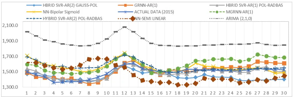
Respectively, the forecasting performance obtained by FFNN with different numbers of hidden nodes is depicted in Fig. 2. From this figure, we can see that FFNN requires different numbers of hidden nodes for different datasets to obtain good performance.
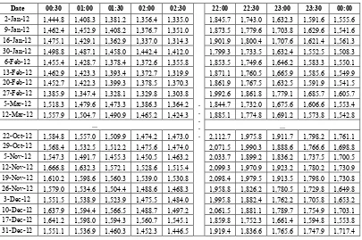
TABLE I. EXAMPLE THE DATASET ELECTRIC LOAD DURING NATIONAL HOLIDAY SEASON 2012
Date 00:30 01:00 01:30 02:00 02:30
. . . . .
22:00 22:30 23:00 23:30 00:00
2-Jan-12 1,444.8 1,408.3 1,381.2 1,356.4 1,335.0 1,845.7 1,743.0 1,632.3 1,591.6 1,555.6
9-Jan-12 1,462.4 1,452.9 1,408.2 1,376.7 1,351.0 1,873.5 1,779.6 1,703.8 1,629.6 1,541.6
16-Jan-12 1,475.1 1,429.1 1,362.9 1,337.0 1,314.3 1,901.9 1,800.4 1,707.6 1,621.4 1,561.3
30-Jan-12 1,498.8 1,487.1 1,458.0 1,442.4 1,412.0 1,799.3 1,733.5 1,632.4 1,552.5 1,508.3
6-Feb-12 1,455.4 1,428.7 1,378.4 1,372.6 1,355.8 1,853.5 1,749.6 1,646.2 1,583.3 1,550.1
13-Feb-12 1,462.9 1,423.3 1,393.4 1,372.7 1,319.9 1,871.1 1,760.5 1,665.9 1,585.6 1,549.9
20-Feb-12 1,452.7 1,422.3 1,399.3 1,378.5 1,370.3 1,861.9 1,767.5 1,632.5 1,591.9 1,541.5
27-Feb-12 1,385.9 1,347.4 1,328.1 1,329.8 1,303.8 1,992.6 1,861.8 1,779.1 1,685.7 1,605.7
5-Mar-12 1,518.3 1,479.6 1,473.3 1,386.3 1,364.2 1,844.7 1,732.0 1,675.6 1,606.6 1,553.4
12-Mar-12 1,557.9 1,504.7 1,490.9 1,465.2 1,424.3 1,885.1 1,774.8 1,691.2 1,573.8 1,542.8
... ...
22-Oct-12 1,584.8 1,557.0 1,509.9 1,474.2 1,473.0 2,112.7 1,975.8 1,911.7 1,798.2 1,761.1
29-Oct-12 1,568.4 1,532.5 1,512.2 1,475.6 1,474.0 2,071.5 1,990.3 1,888.6 1,766.6 1,698.8
5-Nov-12 1,547.3 1,491.7 1,455.3 1,450.5 1,463.2 2,033.7 1,899.2 1,836.2 1,737.5 1,700.5
12-Nov-12 1,666.8 1,632.3 1,572.1 1,528.6 1,515.4 2,099.3 1,970.9 1,923.2 1,780.2 1,730.9
19-Nov-12 1,610.2 1,598.6 1,560.3 1,539.0 1,530.8 2,098.4 1,979.5 1,913.5 1,798.0 1,730.8
26-Nov-12 1,579.0 1,534.6 1,504.4 1,488.6 1,468.3 1,958.8 1,826.2 1,780.5 1,729.8 1,649.8
3-Dec-12 1,551.5 1,538.9 1,523.9 1,475.5 1,484.0 1,995.8 1,882.4 1,762.2 1,705.8 1,653.2
10-Dec-12 1,637.9 1,594.4 1,566.5 1,488.7 1,497.2 2,061.5 1,881.1 1,789.7 1,754.9 1,703.1
17-Dec-12 1,641.2 1,598.0 1,594.3 1,560.7 1,545.1 1,859.8 1,752.3 1,661.4 1,594.8 1,553.8
TABLE II. COMPARING MODELS
MODEL Type of Parameter and Optimization Accuracy
Classical Time Series ARIMA (2,1,0) Parameter AR1=0.8030 AR2=-0.2008 R2 60,44%
HYBRID-SVR-AR(1) Combination of Kernel Gaussian + Kernel Radial Basis with Optimization
Quadratic 0.0219
R2 90,44%
Combination of Kernel Polynomial + Kernel Radial Basis with Optimization Cross Validation : Cost=10; Epsilon=0.0001
R2 98,74
HYBRID-SVR-AR(2) Combination of Kernel Gaussian + Kernel Polynomial with Optimization SMO R297,19%
Combination of Kernel Polynomial + Kernel Radial Basis with Optimization MOSEK
R2 95,27%
Neural Network (12 Input Layer, 12 Hidden Layer) Bipolar sigmoid with Optimization Cross Validation :Validation Ratio 0.2 ; PQ Threshold 1.5 and strip 5
R2 96,56%
Neural Network (12 Input Layer, 12 Hidden Layer) Semi Linear with Optimization Cross Validation : Validation Ratio 0.2 ; PQ Threshold 1.5 and strip 5
R2=95,17%
Neural Network (12 Input Layer, 12 Hidden Layer) SIGMOID with Optimization Cross Validation: Validation Ratio 0.2 ; PQ Threshold 1.5 and strip 5
R2=80,09%
Neural Network (12 Input Layer, 12 Hidden Layer) Hyperbolic Tangent with Optimization Cross Validation: Validation Ratio 0.2 ; PQ Threshold 1.5 and strip 5
R2=87,86%
Neural Network (6 Input Layer, 6 Hidden Layer) Bipolar sigmoid with Optimization Cross Validation: Validation Ratio 0.2 ; PQ Threshold 1.5 and strip 5
R2=84,69%
Neural Network (6 Input Layer, 6 Hidden Layer) Semi Linear with Optimization Cross Validation: Validation Ratio 0.2 ; PQ Threshold 1.5 and strip 5
R2=85,74%
Neural Network (6 Input Layer, 6 Hidden Layer) SIGMOID with Optimization Cross Validation: Validation Ratio 0.2 ; PQ Threshold 1.5 and strip 5
R2=83,73%
Neural Network (6 Input Layer, 6 Hidden Layer) Hyperbolic Tangent with Optimization Cross Validation: Validation Ratio 0.2 ; PQ Threshold 1.5 and strip 5
R2=85,24%
Generalized Regression Neural Network (GRNN) – AR 1 Radial Basis Function R2 96,76%
Generalized Regression Neural Network (GRNN) – AR 2 Radial Basis Function R289,88%
Modified Generalized Regression Neural Network (M-GRNN) – AR 1
Radial Basis Function R2 96,43%
Modified Generalized Regression Neural Network (M-GRNN) – AR 2
Radial Basis Function R2 87,77%
We aim to demonstrate not only that SVR performs well with the number of examples, but also that it performs well against the number of kernels and function activation in neural network. Kernels are useful for training a model, but there is one flaw: we do not know what that model should return if we pass in an example that we have not seen yet. In the fact that the characteristic property of a time series data is not generated independently, their dispersion varies in time, They have cyclic components and often governed by a trend.
Statistical procedures that suppose independent and identically distributed data are, therefore excluded from the analysis of time series. After doing a combination of methods can be found that. HYBRID-SVR-AR (1) with the combination of Kernel Polynomial + Kernel Radial Basis with Optimization Cross Validation is the best model for forecasting on electric load in 2015 also modified generalized regression neural network (MGRNN). The main idea of Cross Validation (CV) is to divide data into two parts (once or several times): one (the training set) used to train a model and the other (the validation set) used to estimate the error of the model. CV selects the parameter among a group of candidates with the smallest CV error, where the CV error is the average of the multiple validation errors. Normally, K fold, leave-one-out, or repeated random sub-sampling procedures were used for CV. Basically, the efficient kernels have been proposed to tackle the challenges in time series through kernel machines. Based on table 1 comparing model, it was found that the
combination of polynomial and radial basis has excellent performance with Cost(C) = 10; Epsilon = 0.0001. Once the kernel function is specified, and the parameters are then used to map the training data. The polynomial kernel function with d=1 can be defined
Moreover, we get the kernel equation as follows and used for data training mapping:
In predicting the SVR equation by finding the beta value with tolerance = beta > C *10-6, It suppose in the first point beta
value = 0.4974*10-6 > tolerance then the first point is called
the support vector and is used in forming the prediction equation. The number of support vectors that formed is 144 data. It means 144 data is a support vector and used in the equation to predict electrical power load. The next beta value is used in the SVR equation to predict the data testing. Furthermore, based on the results of values and are incorporated into the following equations
Fig. 2. Forecasting Performance
IV.CONCLUSION
In case of knowledge mining from the data and also improve the accuracy of the forecast we combine the traditional time series techniques of ARIMA with machine learning as well as Feed Forward Neural Network (FFNN), Generalized Regression Neural Network (GRNN), and support vector regression with the combination of kernel Gaussian, polynomial, and radial basis. We get high accuracy with R2
more than 80%. Although the combination of multi-kernel provides good results but requires high computational complexity. This work could be extended by using Group Method Data Handling (GMDH) in prediction and short-term forecasting
ACKNOWLEDGMENT
This research supported by School of Mathematical Sciences the National University of Malaysia and Bioinformatics and Data Science Research Center (BDSRC) Bina Nusantara University.
REFERENCES
[1] T. Hong, “Short Term Electric Load Forecasting,” North Carolina State University, 2010.
[2] D. Genethliou, “Statistical Approaches to Electric Load
Forecasting,” Stony Brook University, 2015.
[3] W. Y. Zhang, W. C. Hong, Y. Dong, G. Tsai, J. T. Sung, and G.
feng Fan, “Application of SVR with chaotic GASA algorithm in cyclic electric load forecasting,” Energy, vol. 45, no. 1, pp. 850– 858, 2012.
[4] L. Datong, P. Yu, and P. Xiyuan, “Fault prediction based on time series with online combined kernel SVR methods,” in 2009 IEEE Intrumentation and Measurement Technology Conference, I2MTC 2009, 2009, pp. 1167–1170.
[5] M. Karasuyama and R. Nakano, “Optimizing SVR hyperparameters via fast cross-validation using AOSVR,” in IEEE International Conference on Neural Networks - Conference Proceedings, 2007, pp. 1186–1191.
[6] R. E. Caraka, H. Yasin, and A. W. Basyiruddin, “Peramalan Crude Palm Oil ( CPO ) Menggunakan Support Vector Regression Kernel
Radial Basis,” Matematika, vol. 7, no. 1, pp. 43–57, 2017. [7] A. I. McLeod, H. Yu, and E. Mahdi, “Time Series Analysis with R,”
Handb. Stat., vol. 30, no. February, pp. 1–61, 2011.
[8] A. Harvey and V. Oryshchenko, “Kernel density estimation for time
series data,” Int. J. Forecast., vol. 28, no. 1, pp. 3–14, 2012. [9] S. Rüping, “SVM Kernels for Time Series Analysis,” Univ.
Dortmund, p. 8, 2001.
[10] W. Chu and S. S. Keerthi, “Support vector ordinal regression.,”
Neural Comput., vol. 19, no. 3, pp. 792–815, 2007.
[11] A. J. Smola, B. Sch, and B. Schölkopf, “A Tutorial on Support
Vector Regression,” Stat. Comput., vol. 14, no. 3, pp. 199–222, 2004.
[12] J. Nocedal and S. J. Wright, “Quadratic Programming,” Numer. Optim., no. Chapter 18, pp. 448–496, 2006.
[13] L. Bai, J. E. Mitchell, and J. S. Pang, “Using quadratic convex reformulation to tighten the convex relaxation of a quadratic
program with complementarity constraints,” Optim. Lett., vol. 8, no. 3, pp. 811–822, 2014.
[14] H. Drucker, C. Burges, L. Kaufman, A. Smola, and V. Vapnik,
“Support Vector Regression Machines,” Neural Inf. Process. Syst., vol. 1, pp. 155–161, 1996.
[15] C. Cortes and V. Vapnik, “Support-Vector Networks,” Mach. Learn., vol. 20, no. 3, pp. 273–297, 1995.
[16] R. I. Rasel, N. Sultana, and P. Meesad, “An efficient modelling approach for forecasting financial time series data using support
vector regression and windowing operators,” Int. J. Comput. Intell. Stud., vol. 4, no. 2, 2015.
[17] Y. Bai and C. Li, “Daily natural gas consumption forecasting based on a structure-calibrated support vector regression approach,”
Energy Build., vol. 127, no. November, pp. 571–579, 2016. [18] H. Yasin, R. E. Caraka, Tarno, and A. Hoyyi, “Prediction of crude
oil prices using support vector regression (SVR) with grid search -
Cross validation algorithm,” Glob. J. Pure Appl. Math., vol. 12, no. 4, 2016.
[19] F. Tang, “Kernel Methods For Time Series Data,” The University of Birmingham, 2015.
[20] R. E. CARAKA, “Pemodelan General Regression Neural Network
(GRNN) Dengan Peubah Data Input Return Untuk Peramalan Indeks Hangseng,” in Trusted Digital Indentitiy and Intelligent System, 2014, pp. 283–288.
[21] R. Caraka and H. Yasin, “Prediksi Produksi Gas Bumi Dengan
General Regression Neural Network (Grnn).” Jurusan Statisitka
Unpad, Bandung, 2015.
[22] R.E. Caraka, H. Yasin, and P. A, “Pemodelan General Regression Neural Network ( Grnn ) Dengan Peubah Input Data Return Untuk Peramalan Indeks Hangseng,” no. Snik, 2014.