Full Terms & Conditions of access and use can be found at
http://www.tandfonline.com/action/journalInformation?journalCode=ubes20
Download by: [Universitas Maritim Raja Ali Haji] Date: 11 January 2016, At: 23:20
Journal of Business & Economic Statistics
ISSN: 0735-0015 (Print) 1537-2707 (Online) Journal homepage: http://www.tandfonline.com/loi/ubes20
Tilted Nonparametric Estimation of Volatility
Functions With Empirical Applications
Ke-Li Xu & Peter C. B. Phillips
To cite this article: Ke-Li Xu & Peter C. B. Phillips (2011) Tilted Nonparametric Estimation of
Volatility Functions With Empirical Applications, Journal of Business & Economic Statistics, 29:4, 518-528, DOI: 10.1198/jbes.2011.09012
To link to this article: http://dx.doi.org/10.1198/jbes.2011.09012
Published online: 24 Jan 2012.
Submit your article to this journal
Article views: 287
View related articles
Tilted Nonparametric Estimation of Volatility
Functions With Empirical Applications
Ke-Li X
UDepartment of Economics, Texas A&M University, College Station, TX 77843-4228 (keli.xu@econmail.tamu.edu)
Peter C. B. P
HILLIPSDepartment of Economics, Cowles Foundation for Research in Economics, Yale University, P. O. Box 208281, New Haven, CT 06520; The University of Auckland Business School, Auckland 1142, New Zealand; School of Social Sciences, University of Southampton, Southampton, SO17 1BJ, United Kingdom; School of Economics, Singapore Management University, Singapore 178903 (peter.phillips@yale.edu)
This article proposes a novel positive nonparametric estimator of the conditional variance function without reliance on logarithmic or other transformations. The estimator is based on an empirical likelihood mod-ification of conventional local-level nonparametric regression applied to squared residuals of the mean regression. The estimator is shown to be asymptotically equivalent to the local linear estimator in the case of unbounded support but, unlike that estimator, is restricted to be nonnegative in finite samples. It is fully adaptive to the unknown conditional mean function. Simulations are conducted to evaluate the finite-sample performance of the estimator. Two empirical applications are reported. One uses cross-sectional data and studies the relationship between occupational prestige and income, and the other uses time series data on Treasury bill rates to fit the total volatility function in a continuous-time jump diffusion model.
KEY WORDS: Conditional heteroscedasticity; Conditional variance function; Empirical likelihood; Heteroscedastic nonparametric regression; Jump diffusion; Local linear estimator.
1. INTRODUCTION
Conditional variance estimation is important in many appli-cations. It is crucial in inference for the parameters in the con-ditional mean function. For example, to test for the causal treat-ment effect in a regression discontinuity design (Hahn, Todd, and Van der Klaauw2001; Porter2003; Imbens and Lemieux 2008), the conditional variances of the outcome variable on the running variable at the threshold have to be estimated. In a time series context, Hansen (1995) obtained generalized least squares-type efficient estimators of parameters in the mean function by incorporating nonparametric conditional variance estimates (see also Xu and Phillips2008). Conditional variance estimation is also a key intermediate step in estimating some economic or financial quantities of practical importance. In a recent study, Martins-Filho and Yao (2007) proposed a non-parametric method to estimate a production frontier function starting from estimation of the conditional variance of the out-put given the inout-put. Shang (2008) provided a two-stage value-at-risk forecasting procedure in a nonparametric ARCH frame-work based on preliminary estimation of the volatility function (viz. the conditional standard deviation) and then quantile esti-mation using the devolatized residuals.
When the conditional variance is modeled nonparametrically, as in the applications mentioned earlier, the estimation methods that are commonly recommended are based on local polyno-mial estimation, among which local linear estimation is espe-cially popular because of its attractive properties. The theoreti-cal foundation for this approach has been developed by Ruppert et al. (1997) and Fan and Yao (1998), among others. However, one drawback of the local linear variance estimator, which does not apply to the local linear mean function estimator, is that it
may give negative values in finite samples, which makes volatil-ity estimation impossible. Negative variance estimates may oc-cur for large or small smoothing bandwidths and are frequently observed at design points around which observations are rela-tively sparse. Consequently, it is commonly recommended in applications to use the theoretically less satisfactory local con-stant estimator (also known as the Nadaraya–Watson estimator) when fitting the variance function (Chen and Qin2002; Porter 2003).
In this article we propose a new volatility function estimator that is almost asymptotically equivalent to the local linear es-timator but is guaranteed to be nonnegative. Our eses-timator has the same asymptotic bias and variance as the local linear esti-mator when the explanatory variable has unbounded support. Such equivalence is important, because it allows extension of efficiency arguments along the lines of those of Fan (1992) for the local linear estimator to our new procedure. It also is conve-nient in that the mean squared error (MSE) or integrated MSE-based selection criteria for a global or local variable smoothing bandwidth for the local linear estimator continue to apply. The new volatility function estimator is based on the idea of adjust-ing the conventional local constant estimator by minimally tilt-ing the empirical distribution subject to a discrete bias-reductilt-ing moment condition satisfied by the local linear estimator (Hall and Presnell1999). The resultantreweighted local constant es-timator, ortilted estimator, inherits the nonnegativity restriction of the variance function from the usual local constant estima-tor while preserving the superior bias, boundary correction, and
© 2011American Statistical Association Journal of Business & Economic Statistics
October 2011, Vol. 29, No. 4 DOI:10.1198/jbes.2011.09012
518
minimax efficiency properties of the local linear estimator. We also show the adaptiveness of this procedure to the unknown mean function; that is, it estimates the volatility function as ef-ficiently as if the true mean function were known.
Ziegelmann (2002) recently obtained a nonnegative nonpara-metric volatility estimator by fitting an exponential function lo-cally (rather than a linear function as in the local linear estima-tor) within the general locally parametric nonparametric frame-work of Hjort and Jones (1996) (see also Yu and Jones2004) in a Gaussian iid setting. This estimator is not equivalent to the local linear estimator, and it essentially estimates the logarithm of the variance rather than the variance itself, thereby leading to an additional bias term.
The remainder of the article is organized as follows. Sec-tion 2.1 describes the nonparametric heteroscedastic regres-sion model, the framework within which the reweighted local constant volatility estimator is introduced in Section2.2. Sec-tion 2.3presents the asymptotic distributional theory for sta-tionary and mixing time series for both interior and boundary points, and suggests a consistent estimator of the asymptotic variance. Section3evaluates the finite-sample performance of the proposed estimator via simulations. Section4reports two empirical applications, a study of the volatility of the relation-ship between income and occupational prestige in Canada using cross-sectional data and an estimation of the total volatility of 90-day Treasury bill yields in the context of a continuous-time jump diffusion model. Section5 concludes and presents some extensions. Proofs are collected in theAppendix.
2. MAIN RESULTS
2.1 The Heteroscedastic Regression Model
We focus on the following nonparametric heteroscedastic re-gression model:
left unspecified and are the focus of statistical investigation. The reader should keep in mind that our proposed volatility estimator applies straightforwardly to the mean-0 case, for ex-ample, the nonparametric ARCH model whenXt=Yt−1 (Pa-gan and Schwert 1990; Pagan and Hong 1991). Many non-parametric economic models can be cast within the frame-work (1). Martins-Filho and Yao (2007) presented a recent application in stochastic frontier analysis, and Hahn, Todd, and Van der Klaauw (2001), Porter (2003), and Imbens and Lemieux (2008) addressed the analysis of causal treatment ef-fects. The model (1) is also of fundamental importance in finan-cial econometrics because of its ability to allow for nonlinearity and conditional heteroscedasticity in financial time series mod-eling. It also can be considered the discretized version of the nonparametric continuous-time diffusion model that is com-monly used in financial derivative pricing (Ait-Sahalia1996; Stanton1997; Bandi and Phillips2003).
2.2 The Conditional Variance Estimator
Our nonparametric estimator of the conditional variance functionσ2(·)is residual-based, which relies on first-stage non-parametric estimation of the conditional mean function m(·). Let W(·) and K(·) be kernel functions and h′ =h′(n),h= h(n) >0 be smoothing bandwidths that determine model com-plexity. Following recommendations in the theoretical and em-pirical literature, we can fitm(·)using the local linear method that solves Application of different bandwidths in mean and variance es-timation has been stressed by several authors (Ruppert et al. 1997; Yu and Jones2004). In what follows, we useh′for mean regression estimation andhfor variance estimation.
To estimate the conditional variance functionσ2(x), instead of fitting the squared residualsrt2= [Yt−m(Xt)]2toXtusing a
second-stage local linear smoother, as was done by Ruppert et al. (1997) and Fan and Yao (1998), we consider the following reweighted local constant estimator:
wherewt(x)solves the constrained optimization problem
{w1(x), . . . ,wn(x)}
is considered the key condition for local linear estimation to achieve bias reduction (see Fan and Gijbels1996). Without (6), the optimization problem (4)–(5) is solved by the uniform weights wUNIFt (x)=1/n for all t, which reduces (3) to the usual local constant estimator (or the Nadaraya–Watson esti-mator). Thus the reweighted local constant estimator (3) ef-fectively minimizes the distance to the local constant estimator while preserving the bias-reducing condition of the local linear estimator. The distance used here is Kullback–Leibler diver-gence, although other distance measures can be used (Cressie and Read1984) and has an important connection to the empiri-cal likelihood approach of Owen (2001).
Computationally, the reweighted estimator is very easy to use in practice, because (4) can be solved by any empirical likeli-hood maximization program. To be specific, the weightswt(x)
in (3) can be obtained via the Lagrange multiplier method, that is,
where the Lagrange multiplierλsatisfies
n
t=1
[1+λ(Xt−x)Kh(Xt−x)]−1(Xt−x)Kh(Xt−x)=0. (8)
The reweighting idea is due to the intentionally biased boot-strap of Hall and Presnell (1999). It is especially powerful for conditional variance estimation, because the associated esti-mates always fall within the range[min1≤t≤nr2t,max1≤t≤nr2t],
thereby ensuring nonnegative results. The restriction in (6) is used, so that the original estimator (i.e., the local constant es-timator) is modified to the smallest extent necessary to main-tain the attractive properties of the local linear estimator. We can expand (6) so that the resulting variance estimator satis-fies other desirable properties. For example, we can also impose the constraint d[σ2(x)]/dx≥0 or d2[σ2(x)]/dx2≥0 to ensure monotonicity (Hall and Huang2001) or convexity of the esti-mated variance function as may be needed.
The reweighting idea has been used fruitfully in other con-texts, for example, by Hall, Wolff, and Yao (1999) for monotone estimation of the conditional distribution function that is within the range[0,1], by Cai (2002) for monotone conditional quan-tile estimation, and by Xu (2010) for nonnegative diffusion functional estimation in a continuous-time nonstationary dif-fusion model.
2.3 Limit Theory
The asymptotic distribution of the reweighted local con-stant estimator of the conditional variance function is given in the following theorem for both interior and boundary spa-tial points. Letf(·)be the stationary density function ofXtand
¨
σ2(z)=d2[σ2(z)]/dz2.Assume that the kernel functionsW(·) andK(·)are symmetric density functions each with bounded support[−1,1].
Theorem 1. (a) Suppose thatxis such that x±h is in the support off(x). Under the assumptions stated in theAppendix, asn→ ∞, is a constant such that 0<c<1. Under the assumptions stated in theAppendix, asn→ ∞,
Remark 1. In Theorem 1, part (a) is concerned with inte-rior points when f has bounded support or the case where f has unbounded support, and part (b) is concerned with bound-ary points. The theorem shows that the reweighted local con-stant variance estimator is asymptotically equivalent to the lo-cal linear variance estimator (cf. Ruppert et al.1997; Fan and Yao1998), except for different scale constants for the bias and the variance at boundary points. The condition (6) is effec-tive in removing a bias term of order Op(h2) in the interior
and a bias term of orderOp(h) on the boundary of the local
constant estimator. Thus no additional boundary correction is needed. The following heuristic argument helps elucidate this feature. The bias ofσ2(x)is approximately accounted for by the term(nh)−1nt=1pt(x)K((Xt−x)/h)[σ2(Xt)−σ2(x)],where
pt(x)= [ n
t=1wt(x)K((Xt −x)/h)]−1wt(x); see the proof of
Theorem1in theAppendix. By a second-order Taylor expan-sion ofσ2(Xt)atxand the discrete moment condition (6),
if x is in the interior
h2f(a)K1σ¨2(a+ch)/2+op(h2),
if x is on the left boundary
h2f(b)K1σ¨2(b−ch)/2+op(h2),
if x is on the right boundary.
The bias term of orderOp(h)is removed by the condition (6) for
anynboth at interior and boundary points just as for the local linear smoother. It is essentially different from the conventional local constant estimator, for which the bias term of orderOp(h)
is eliminated in the limit via symmetry of the kernel function for interior points but does not vanish for boundary points.
Remark 2. The constantsλcandλcdecrease withcand
ap-proach 0 when c→1. Theorem1(ii) also holds for an inte-rior pointxby noting that K0=K0=1, K1=K1=K1 and K2=K2=K2whenc∈ [1, (b−a)/2h].
Remark 3. When the true mean functionm(·)is known, the reweighted local constant conditional variance estimator fol-lows from Cai (2001) with the outcome variable[Yt−m(Xt)]2,
because σ2(x)=E[(Yt−m(Xt))2|Xt =x]. Theorem 1 shows
that the residual-based estimatorσ2(·), which does not require m(·)to be known, is asymptotically as efficient as the oracle es-timator, which assumes knowledge ofm(·). This adaptiveness property to the unknown conditional mean function is shared by other residual-based variance estimators (see Fan and Yao 1998; Ziegelmann2002).
Remark 4. Implementation of the reweighted volatility esti-mator involves determination of the amount of smoothing, that is, selection of the smoothing bandwidthh. Theorem1shows that minimization of the asymptotic mean squared error (MSE) or integrated MSE (IMSE) leads to an optimal local bandwidth or global bandwidth of the formh=ςn−1/5,whereς involves nuisance parameters f(x), σ2(x),σ¨2(x),ξ2(x), and constants related to the kernel function. A feasible bandwidth is usually obtained by estimating ς by, for example, parametric fitting (the rule of thumb), iterations (the plug-in method) or cross-validation. An attractive feature of the reweighted estimator is that given its asymptotic equivalence to the local linear estima-tor, as implied by Theorem1, the asymptotic MSE- or IMSE-based bandwidth selection criteria for the local linear estimator (see Fan and Yao1996) generally apply to the reweighted esti-mator as well.
Remark 5. Härdle and Tsybakov (1997) studied a volatil-ity estimator for the model (1) assuming thatXt=Yt−1based on differencing the local polynomial estimators of the second conditional moment and the squared first conditional moment. Their estimator is not nonnegative and, as noted by Fan and Yao (1998), is not fully adaptive to the mean function. Ziegelmann’s (2002) nonnegative residual-based local exponential (LE) vari-ance estimator is obtained asσLE2 =exp(ψ1), where(ψ1, ψ2) = arg min(ψ1,ψ2)
n
t=1[rt2−exp(ψ1+ψ2(Xt−x))]2K((Xt−x)/h).
It belongs to a large class of local nonlinear estimators (Hjort and Jones1996; Gozalo and Linton2000). To ensure nonneg-ativity of the resultant variance estimator, the procedure effec-tively approximates the logarithm of the variance (instead of the variance itself) locally by a linear function, thereby introducing an extra bias term.
Remark 6. The asymptotic variance ofσ2(x)can be consis-tently estimated both at interior and boundary points, thereby allowing construction of consistent pointwise confidence inter-vals. Let (x) = f−2(x)V(x) where V(x) = nh−1 ×
n
t=1K2((Xt−x)/h)[r2t−σ2(x)]2andf(x)=h−1 n
t=1K((Xt−
x)/h).
Theorem 2. (a) Under the conditions of Theorem 1(a), as n→ ∞,(x)→p K2σ4(x)ξ2(x)/f(x);
(b) Under the conditions of Theorem1(b), asn→ ∞,(a+ ch) →p K2σ4(a)ξ2(a)/[K
2
0f(a)] and (b − ch)
p
→
K2σ4(b)ξ2(b)/[K20f(b)].
The following two sections provide several numerical exam-ples illustrating the use of the new volatility estimator with simulated and real data. In all applications, the Epanechnikov functionK(u)=0.75(1−u2)I(−1,1)is used for both kernelsW andK, and the bandwidth parameter in mean estimationh′ is selected by least squares cross-validation.
Figure 1. The means, 10% quantiles and 90% quantiles of the LC, LL, RLC, and LE estimates of the volatility functionσ2(x)=1+0.4x2
in the AR-ARCH model (11) whenφ=0 over 1000 replications, using the smoothing bandwidthh=0.7.
3. SIMULATIONS
The finite-sample performance of the proposed estimator is assessed in the following simple time series setting. We gener-aten+201 observations from the AR-ARCH model:
Yt=φYt−1+
ρ0+ρ1Yt2−1εt (11)
with(ρ0, ρ1)=(1,0.4),Y1=0, φ∈ {0,0.4}, andεt
iid
∼N(0,1).
The first 200 observations are dropped to eliminate initializa-tion effects, so the sample size isn.The heteroscedastic regres-sion model (1) is then estimated with the generated data. Note that (11) is different from the ARCH(1) model regardless of the true value of φ , because it allows for uncertainty in the mean function. Figures1and2focus on the case whereφ=0.
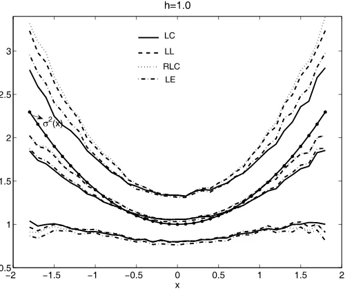
Figure 2. The means, 10% quantiles and 90% quantiles of the LC, LL, RLC, and LE estimates of the volatility functionσ2(x)=1+0.4x2
in the AR-ARCH model (11) whenφ=0 over 1000 replications, using the smoothing bandwidthh=1.0.
Table 1. Frequencies of negative local linear conditional variance estimates in the AR-ARCH model (11) whenφ=0 over 1000
replications (zeros for blank cells)
Bandwidth h=0.7 h=0.6 h=0.5 h=0.4 h=0.3 h=0.2
x=1.8 3 4 6 13 19 61
x=1.6 2 3 3 16 39
x=1.4 1 4 18
x=1.2 6
x=1.1 1 8
x=1.0 8
x=0.9 6
x=0.8 2
We plot the averages, 10% quantiles, and 90% quantiles (over 1000 replications) of the reweighted local constant (RLC) con-ditional variance estimates (whenn=100) at 37 equally spaced spatial points fromx= −1.8 tox=1.8,a range that is wide enough to cover most spatial points the time series visits. For comparison, we also plot the corresponding results for the local constant (LC), local linear (LL) and Ziegelmann’s (2002) lo-cal exponential (LE) estimators along with the true conditional variance function. In the two figures, the smoothing bandwidths h=0.7 and 1.0 are chosen to illustrate the bandwidth effects. The common bandwidth effects are observed; a larger band-width generally reduces the variability but increases the bias of the estimate.
A striking finding is that the RLC estimator has an overall performance very close to that of the LL estimator for all spatial points considered in terms of both bias and variability. This is not surprising, given the asymptotic similarity (and equivalence for unbounded support) of the two methods. But in particular samples, negative LL variance estimates are found (with fre-quencies listed in Table1) mainly at spatial points with sparse neighborhoods or when a small bandwidth is used, in which case the estimates fluctuate widely. In such cases, of course, the volatility estimates are effectively useless. On the other hand, the LC and LE estimators generally suffer from large biases, especially at spatial points with relatively fewer observations in their neighborhoods, for example,xwith|x| ≥1.
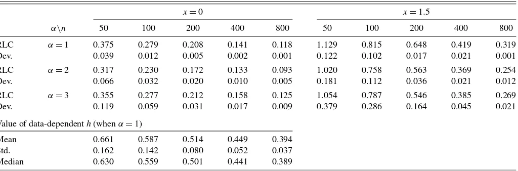
We also consider the case with serial correlation inYt,(i.e.,
φ=0.4), and we find that the results reported earlier are quite robust to weak serial correlation. Table2 reports the MSEs of the RLC volatility estimates when the data-dependent band-widths are used, that is,h=αsn−1/5, wheresis the standard deviation of the sample andα∈ {1,2,3}.The MSEs decrease when the sample size increases, and they are larger for the de-sign pointx=1.5, where the process visits sparingly, than for x=0, where the process visits more frequently. The bandwidth withα=2 appears to work best in this setting and generally gives the smallest MSEs compared with the other two band-widths. The distribution of the values of the data-dependent bandwidths is described in Table2; for example, the median of the bandwidths (over 1000 replications) whenn=100 and α=2 is 0.559×2=1.118. Table2also reports the deviation of the MSE of the RLC volatility estimate from that of the esti-mate based on the true mean functionm(x)=0.4x. As the sam-ple size increases, the deviation approaches 0, and the effects of estimating the unknown mean function on volatility estimation disappear asymptotically, thereby confirming the adaptiveness property suggested by the limit theory.
4. EMPIRICAL APPLICATIONS
This section provides two empirical examples to illustrate the usefulness of our proposed methodology. The first is a cross-sectional data application, and the second involves financial time series.
4.1 Occupational Prestige versus Income
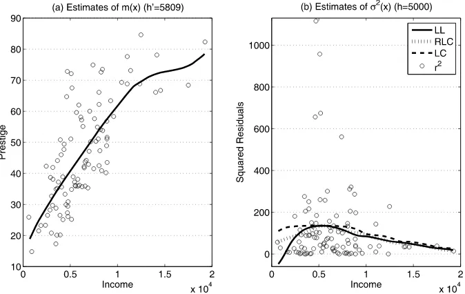
Fox (2002) studied the relationship between occupational prestige and the average income of Canadian occupations. The dataset is available in thecarpackage of R(R Development Core Team2010) designatedPrestige.It consists of cross-sectional observations for 102 occupations. Prestige for each occupation is measured by the Pineo–Porter prestige score from a social survey. Figure3(a) shows a scatterplot and a local lin-ear mean fit with the bandwidthh′=5809 chosen via cross-validation (Li and Racine2004; see also Li and Racine2007, p. 93). It also might be useful to provide variance estimates, for
Table 2. MSEs of the RLC volatility estimates and the adaptiveness to the unknown mean function in the AR-ARCH model (11) whenφ=0.4 (Dev. represents the deviation of the MSE of the RLC volatility estimate from that of the estimate based on the true mean function)
x=0 x=1.5
α\n 50 100 200 400 800 50 100 200 400 800
RLC α=1 0.375 0.279 0.208 0.141 0.118 1.129 0.815 0.648 0.419 0.319
Dev. 0.039 0.012 0.005 0.002 0.001 0.122 0.102 0.017 0.021 0.001
RLC α=2 0.317 0.230 0.172 0.133 0.093 1.020 0.758 0.563 0.369 0.254
Dev. 0.066 0.032 0.020 0.010 0.005 0.181 0.112 0.036 0.021 0.012
RLC α=3 0.355 0.277 0.212 0.158 0.125 1.054 0.787 0.546 0.385 0.269
Dev. 0.119 0.059 0.031 0.017 0.009 0.379 0.286 0.164 0.045 0.021
Value of data-dependenth(whenα=1)
Mean 0.661 0.587 0.514 0.449 0.394
Std. 0.162 0.142 0.080 0.052 0.037
Median 0.630 0.559 0.501 0.441 0.389
Figure 3. Prestige versus income. (a) Local linear estimation of the conditional mean function using the bandwidthh′=5809;(b) Estimates of the conditional variance function based on the squared residuals using the LL, RLC, and conventional LC methods with the bandwidth
h=5000.
example, for the construction of pointwise confidence intervals for the mean function or some automatic bandwidth selection criteria.
Figure 3(b) plots the squared mean regression residuals against the explanatory variable (average income) and the fit-ted curves that give the functional conditional variance esti-mates by the LC, LL, and RLC methods. The fitted curves are calculated over 186 levels of average incomes equally spaced fromx=711 to 19,211. For illustration, we use the bandwidth h=5000. Clearly the LL variance estimates are negative at small values of average incomes, and the conventional LC esti-mates are always positive but suffer from large biases. Our pro-posed RLC estimates appear to provide a good compromise be-tween those two estimates, and evidently capture the declining variances in a reasonable way (being always positive) when the level of average income is low. At moderate and high levels of average income, for which the data are relatively rich, the RLC variance estimates are very close to the local linear estimates, not surprising given their first-order asymptotic similarity.
This example demonstrates the need to carefully select the bandwidth to avoid the negativity problem when the LL mator is used to estimate variance. We also consider the esti-mated IMSE-based optimal bandwidth via rule of thumb (Fan and Gijbels1996, p. 111) for the LL and RLC variance esti-mators. This has valuehop=1871. We find that this bandwidth
is too small and it gives wiggly estimated curves, necessitating intervention for bandwidth selection. Figure4shows the esti-mated curves whenh=2hop.This poses no problem for the LL
estimator, because the estimated curve is still above the zero line. Our empirical results indicate that further increasing the bandwidth would induce negative variance estimates.
To study the sensitivity of various functional variance esti-mates to the smoothing parameter, we estimate the conditional variance σ2(x) at two levels of average incomes, x=1000 and 6000, using 91 bandwidths equally spaced fromh=1000 to 10,000. The results are shown in Figure5. At the bound-ary pointx=1000,negative estimates arising from the local
linear fit occur within the bandwidth range of approximately (4000, 6000), which might reasonably be chosen by empirical researchers. The RLC estimates generally lie between the LL and the conventional LC estimates and apparently are quite sta-ble over various bandwidths. At the interior pointx=6000,the three fitted values are much closer to one another, and the RLC and LL curves are almost indistinguishable.
4.2 Jump Diffusion Volatilities
The reweighting idea developed in this article also can be used for functional estimation of continuous-time jump
diffu-Figure 4. Prestige versus income. Estimates of the conditional vari-ance function based on the squared residuals using the LL and RLC methods with the bandwidthh=2hop=3742.
Figure 5. Prestige versus income. Estimates of the conditional variance function over 91 bandwidths using LL, RLC and LC methods with design points (a)x=1000 and (b)x=6000.
sions. Jump diffusion models are widely used in finance to ac-count for discontinuities in the sample path. They are more flex-ible than single-factor or multifactor pure diffusion models in generating higher moments that match those typically observed in financial time series (see, e.g., Bakshi, Cao, and Chen1997; Pan2002; Johannes2004).
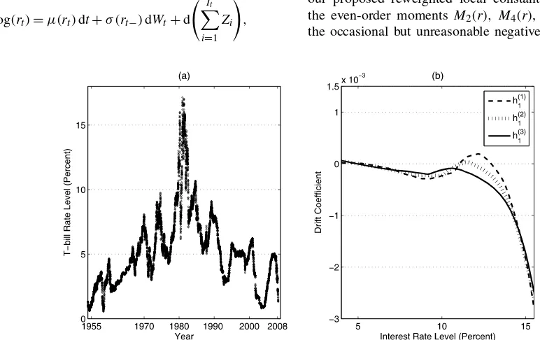
Our empirical application uses T=54 years of daily sec-ondary market quotes for 3-month Treasury bills from Janu-ary 4, 1954, to March 13, 2008, containing n=13,538 ob-servations, plotted in Figure 6(a). The dataset is available from the Board of Governors of the Federal Reserve System (http:// research.stlouisfed.org/ fred2). The spot rate, rt, is
as-sumed to follow the jump diffusion process,
d log(rt)=μ(rt)dt+σ (rt−)dWt+d It
i=1 Zi
,
wherert−=lims↑trs,Wtis a standard Brownian motion,Itis a
doubly stochastic point process with stochastic intensityλ(rt),
andZi
iid
∼N(0, σ2
z).We assume that the mean jump size is 0
without loss of generality. The four values of interest in estima-tion [i.e., the drift funcestima-tionμ(r),the diffusion functionσ2(r), the jump intensityλ(r),for interest rate levelr,and the jump varianceσz2] can be identified for a sufficiently small sampling interval,, by the momentsMj(r)=E(log(rt+/rt)j|rt=r)/
forj=1,2,4,6 using the following approximate moment con-ditions:
M1(r)≃μ(r), M2(r)≃σ2(r)+λ(r)σz2,
M4(r)≃3λ(r)σz4, M6(r)≃15λ(r)σz6.
We use local linear fitting to estimate M1(r), and apply our proposed reweighted local constant method to estimate the even-order moments M2(r), M4(r), and M6(r), to avoid the occasional but unreasonable negative estimates that result
Figure 6. (a) The time series of daily 3-month Treasury bill rates (secondary market rates) from January 4, 1954, to March 13, 2008. (b) Local linear estimators of the drift function using three bandwidths, 3.5%, 4.2%, and 5.0%.
from local linear fitting. The estimates are denoted as Mj(r),
j=1,2,4,6.Based on the daily data,{ri,i=1, . . . ,n}, fol-lowing Johannes (2004), we obtain the estimates step by step:
σz2=n−1
n
i=1
M6(ri)/[5M4(ri)],
λ(r)=M4(r)/(3σz4),
σ2(r)=M2(r)−λ(r)σz2, μ(r)=M1(r).
The jump varianceσz2is first estimated by integrating the ratio of sixth moments to fourth moments over the stationary den-sity with the same bandwidth for the fourth and sixth moments h4=1.7sT−1/5=2.1%,wheres is the standard deviation of the sample. The estimateσz2is 2.39×10⁻³.Then, to estimate λ(r), we consider bandwidths h(4j) =1.2j·h4 (j=0,1,2) in
M4(r). To estimate σ2(r), we use the bandwidth h4 in com-puting M4(r) [and thusλ(r)] and bandwidths h2(j) =1.2jh2 (j=0,1,2)inM2(r), whereh2=1.3sT−1/5=1.7%.Finally, μ(r)is estimated byM1(r)using the bandwidthh1(j)=1.2jh1, j=0,1,2,whereh1=2.8sT−1/5=3.5%.We characterize the bandwidths used in terms of the time spanT (instead of the sample sizen), because the convergence rates of theMj(r)
de-pend onT (or, more generally, on the local time process), as shown by Bandi and Nguyen (2003). The scale constants that we chose are such that the resulting bandwidths are close to those reported in empirical studies of US short rate dynamics.
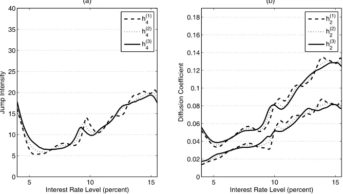
The estimated curvesμ(r),λ(r),σ2(r)are plotted in Fig-ure 6(b) and Figure 7(a) and (b). They are expected to have smaller biases than the estimates of Johannes (2004) and Bandi and Nguyen (2003), which are based on local constant estima-tion of the four moments. Figure7(b) also presents the esti-mates (given in the top three lines) of the total volatility func-tion,σ2(r)+λ(r)σz2.The implication is that for most short rate levels, the diffusion components explain approximately two-thirds of the total volatility and the jump components account for the remaining one-third. This can be compared with the
work of Johannes (2004), who used a subset of our data and found that jumps typically generate more than half the volatil-ity of interest rate changes, and Eraker, Johannes, and Polson (2003) who found that jumps in equity indices explain 10–15 percent of return volatility.
It is noteworthy that limit theories for the local linear and the reweighted local constant estimators of the four moments in the jump diffusion model have not yet become available in the literature. We conjecture that these theories can be studied along the lines of the approach of Bandi and Nguyen (2003). For the pure diffusion models (whereσz2=0), the asymptotic theories for these two methods have been studied by Moloche (2001), Fan and Zhang (2003), and Xu (2010).
5. CONCLUDING REMARKS
This article provides a new nonparametric approach to esti-mating the conditional variance function based on maximizing the empirical likelihood subject to a bias-reducing moment re-striction. The method is fully adaptive for the unknown mean function. The construction of the estimator does not depend on the error distribution, and the estimator is applicable in quite general time series and cross-sectional settings. The estimator preserves the appealing design adaptive, bias, and automatic boundary correction properties of the local linear estimator and is guaranteed to be nonnegative in finite samples. Numerical examples suggest that the new estimator performs well in finite samples and is a promising competitor in estimating conditional variance functions.
Our proposed method can be extended to the case whereXtis
multivariate, for example, in the nonparametric AR-ARCH(p) model, Yt = m(Yt−1, . . . ,Yt−p) + σ (Yt−1, . . . ,Yt−p)εt with Xt =(Yt−1, . . . ,Yt−p)′. In such cases, the constrained
op-timization (4) is conducted under multiple restrictions. To be specific, suppose that we have p covariates, and Xt =
(X1,t, . . . ,Xp,t)′,x=(x1, . . . ,xp)′ arep×1 vectors. The RLC
variance estimator is defined asσ2(x)= [nt=1wt(x)Kh(Xt− x)]−1nt=1wt(x)Kh(Xt−x)rt2 wherert are residuals of a
p-dimensional nonparametric mean fit (e.g., a local linear fit)
Figure 7. (a) Reweighted local constant estimators of the jump intensity using three bandwidths. (b) Reweighted local constant estimators of the second momentM2(r)(the top three lines) and the diffusion coefficient over three bandwidths, respectively.
andKh(Xt−x)=h−ppi=1K((Xi,t−xi)/h)are product kernel
weights. Different bandwidths and kernels could be used for each covariate, but here we assume that they are the same for expositional simplicity. The weightswt(x)are such that (4) is
solved subject to (5) and thep-dimensional restrictions,
n
t=1
wt(x)(Xt−x)Kh(Xt−x)=0. (12)
The local linear weights satisfy (12) and take the form of, for example, whenp=2,wLLt (x)=Ŵ1−Ŵ2(X1,t−x1)+Ŵ3(X2,t−
where det(A) denotes the determinant of the matrix A and
Ŵ(i,j) =nt=1(X1,t −x1)j(X2,t −x2)kKh(Xt −x) for j,k=
0,1,2. Just as in the univariate case, the reweighted estimator selects the weights such that the good bias properties of the local linear estimator are preserved and the resulting variance estimate is always nonnegative.
The foregoing fully nonparametric volatility estimators have slow convergence rates whenpis large, and also pose difficul-ties in interpretation. A popular alternative that can achieve the one-dimensional convergence rate and that imposes reasonably weak assumptions on the specification of the volatility function is the additive model, such as the additive ARCH model con-sidered by Kim and Linton (2004), whereσ (Yt−1, . . . ,Yt−p)=
θ+σ12(Yt−1)+ · · · +σp2(Yt−p). The functions σ12(·), . . . ,
andσp2(·)can be estimated by, for example, marginal integra-tion or backfitting, which essentially involves iterative univari-ate smoothing. Again, the proposed reweighted local constant method is expected to be a promising alternative to the local linear estimator that is commonly recommended.
APPENDIX
This section provides proofs of Theorems1and2. To derive the asymptotic distribution of σ2(x), we make the following assumptions.
Assumptions.
(i) For a given design point x, the functions f(x) >0, σ2(x) >0,E(Y3|X=x)and E(Y4|X=x)are continuous atx, and m(x)¨ =d2m(x)/dx2 and σ¨2(x)=d2(σ2(x))/dx2 are uni-formly continuous on an open set containingx;
(ii) E|Y|4(1+δ)<∞for someδ≥0;
(iii) There exists a constantM<∞such that|g1,t(y1,y2|x1, x2)| ≤Mfor allt≥2,whereg1,t(y1,y2|x1,x2)is the conditional density ofY1andYtgivenX1=x1andXt=x2;
(iv) The kernel functionsW(·)andK(·)are symmetric den-sity functions each with a bounded support[−1,1]. A Lipschitz condition is satisfied by each of functionsf(·),W(·), andK(·);
(v) The process(Xt,Yt)is strictly stationary and absolutely
regular (see, e.g., Davidson1994, p. 209) with mixing coeffi-cientsβ(j)satisfying ∞j=1j2βδ/(1+δ)(j) <∞,whereδ is the
have a computationally convenient representation in (7). For simplicity, we write wt(x) as wt in what follows. Note that rt=Yt−m(Xt)= [m(Xt)−m(Xt)] +σ (Xt)εt, and thus f(x). Because an absolutely regular time series is α-mixing, lemma A2 of Cai (2001) holds under our assumptions, that is, λ= −hK1f′(x)
First, consider the termN2. The denominator ofN2times 1/h is
by (A.3) and an application of Birkhoff’s ergodic theorem (see, e.g., Shiryaev 1996), because E[h−1K((Xt −x)/h)] =
h−1K((u −x)/h)f(u)du→ f(x) as h →0 after a simple change of variables. By a Taylor expansion ofσ2(Xt)atxand
the discrete moment condition (6), the numerator ofN2 times 1/his
× [ ¨σ2(x)(Xt−x)2/2+o((Xt−x)2)]
=h2f(x)K1σ¨2(x)/2+op(h2), (A.5)
by (A.3) and the ergodic theorem. Combining (A.4) and (A.5) givesN2=h2K1σ¨2(x)/2+op(h2).Based on (A.3) and (A.4),
it follows from Fan and Yao [1998, proof of thm. 1(b)–(d)] that
√
First, consider the termN2in (A.2). Note that
h−1
by the ergodic theorem, because
E
ash→0 after a change of variables. By a Taylor expansion of σ2(Xt)ata+chand the discrete moment condition (6),
andN1is asymptotically normal with mean 0 and variance 1/nh times [noting (A.6)],
Thus the desired result follows by (A.2). The case wherex= b−chcan be proved similarly. The proof of (b) is complete.
Proof of Theorem2
Similar to the analysis of the term N1 in the proof of Theo-rem1(a), we have
provided that
by the ergodic theorem. It follows from Fan and Yao (1998) and the proof of Theorem 1(a) that V1j = op(1) for j = and Theorem2(a) follows from (A.4).
(b) This can be proved as in (a) using the arguments given in the proof of Theorem1(b).
ACKNOWLEDGMENTS
The authors thank the editors, the associate editor, two anonymous referees, Donald Andrews, and Taisuke Otsu for helpful comments. Xu acknowledges partial research sup-port from University of Alberta School of Business under an H. E. Pearson fellowship and a J. D. Muir grant. Phillips ac-knowledges partial research support from a Kelly Fellowship and National Science Foundation grants SES 04-142254, 06-47086 and 09-56687.
[Received January 2009. Revised July 2010.]
REFERENCES
Aït-Sahalia, Y. (1996), “Nonparametric Pricing of Interest Rate Derivative Se-curities,”Econometrica, 64, 527–560. [519]
Bakshi, G., Cao, C., and Chen, Z. (1997), “Empirical Performance of Alterna-tive Option Pricing Models,”Journal of Finance, 52, 2003–2049. [524] Bandi, F., and Nguyen, T. (2003), “On the Functional Estimation of
Jump-Diffusion Processes,”Journal of Econometrics, 116, 293–328. [525] Bandi, F., and Phillips, P. C. B. (2003), “Fully Nonparametric Estimation of
Scalar Diffusion Models,”Econometrica, 71, 241–283. [519]
Cai, Z. (2001), “Weighted Nadaraya–Watson Regression Estimation,”Statistics and Probability Letters, 51, 307–318. [521,526,527]
(2002), “Regression Quantiles for Time Series,”Econometric Theory, 18, 169–192. [520]
Chen, S. X., and Qin, Y. (2002), “Confidence Interval Based on a Local Linear Smoother,”Scandinavian Journal of Statistics, 29, 89–99. [518]
Cressie, N., and Read, T. (1984), “Multinomial Goodness-of-Fit Tests,”Journal of the Royal Statistical Society, Ser. B, 46, 440–464. [519]
Davidson, J. (1994),Stochastic Limit Theory: An Introduction for Econometri-cians, Oxford: Oxford University Press. [526]
Eraker, B., Johannes, M., and Polson, N. (2003), “The Impact of Jumps in Volatility and Returns,”Journal of Finance, 58, 1269–1300. [525] Fan, J. (1992), “Design-Adaptive Nonparametric Regression,”Journal of the
American Statistical Association, 87, 998–1004. [518]
Fan, J., and Gijbels, I. (1996),Local Polynomial Modeling and Its Applications, London: Chapman & Hall. [519,521,523]
Fan, J., and Yao, Q. (1998), “Efficient Estimation of Conditional Variance Func-tions in Stochastic Regression,”Biometrika, 85, 645–660. [518-521,527,
528]
Fan, J., and Zhang, C. (2003), “A Re-Examination of Stanton’s Diffusion Es-timations With Applications to Financial Model Validation,”Journal of American Statistical Association, 98, 118–134. [525]
Fox, J. (2002),An R and S-PLUS Companion to Applied Regression, Thousand Oaks: Sage. [522]
Gozalo, P., and Linton, O. (2000), “Local Nonlinear Least Squares: Using Para-metric Information in NonparaPara-metric Regression,”Journal of Economet-rics, 99, 63–106. [521]
Hahn, J., Todd, P., and Van der Klaauw, W. (2001), “Identification and Estima-tion of Treatment Effects With a Regression-Discontinuity Design,” Econo-metrica, 69, 201–209. [518,519]
Hall, P., and Huang, L.-S. (2001), “Nonparametric Kernel Regression Subject to Monotonicity Constraints,”The Annals of Statistics, 29, 624–647. [520] Hall, P., and Presnell, B. (1999), “Intentionally Biased Bootstrap Methods,”
Journal of the Royal Statistical Society, Ser. B, 61, 143–158. [518,520] Hall, P., Wolff, R. C. L., and Yao, Q. (1999), “Methods for Estimating a
Con-ditional Distribution Function,”Journal of the American Statistical Associ-ation, 94, 154–163. [520]
Hansen, B. E. (1995), “Regression With Nonstationary Volatility,” Economet-rica, 63, 1113–1132. [518]
Härdle, W., and Tsybakov, A. B. (1997), “Local Polynomial Estimators of the Volatility Function in Nonparametric Autoregression,”Journal of Econo-metrics, 81, 223–242. [521]
Hjort, N. L., and Jones, M. C. (1996), “Local Parametric Nonparametric Den-sity Estimation,”The Annals of Statistics, 24, 1619–1647. [519,521] Imbens, G. W., and Lemieux, T. (2008), “Regression Discontinuity Designs:
A Guide to Practice,”Journal of Econometrics, 142, 615–635. [518,519] Johannes, M. (2004), “The Statistical and Economic Role of Jumps in
Continuous-Time Interest Rate Models,”Journal of Finance, 59, 227–260. [524,525]
Kim, W., and Linton, O. (2004), “A Local Instrumental Variable Estimation Method for Generalized Additive Volatility Models,”Econometric Theory, 20, 1094–1139. [526]
Li, Q., and Racine, J. S. (2004), “Cross-Validated Local Linear Nonparametric Regression,”Statistica Sinica, 14, 485–512. [522]
(2007),Nonparametric Econometrics: Theory and Practice, New Jer-sey: Princeton University Press. [522]
Martins-Filho, C., and Yao, F. (2007), “Nonparametric Frontier Estimation via Local Linear Regression,”Journal of Econometrics, 141, 283–319. [518,
519]
Moloche, G. (2001), “Local Nonparametric Estimation of Scalar Diffusions,” unpublished manuscript, Boca Raton, FL: MIT. [525]
Owen, A. (2001),Empirical Likelihood, Chapman & Hall/CRC. [519] Pagan, A., and Schwert, G. (1990), “Alternative Models for Conditional Stock
Volatility,”Journal of Econometrics, 45, 267–290. [519]
Pagan, A. R., and Hong, Y. S. (1991), “Nonparametric Estimation and the Risk Premium,” inNonparametric and Semiparametric Methods in Economet-rics and Statistics, eds. W. Barnett, J. Powell, and G. E. Tauchen, Cam-bridge, United Kingdom: Cambridge University Press. [519]
Pan, J. (2002), “The Jump-Risk Premia Implicit in Options: Evidence From an Integrated Time-Series Study,”Journal of Financial Economics, 63, 3–50. [524]
Porter, J. (2003), “Estimation in the Regression Discontinuity Model,” working paper, Dept. of Economics, University of Wisconsin. [518,519]
R Development Core Team (2010),R: A Language and Environment for Statis-tical Computing, Vienna, Austria: R Foundation for Statistical Computing. ISBN 3-900051-07–0, available athttp:// www.R-project.org. [522] Ruppert, D., Wand, M. P., Holst, U., and Hössjer, O. (1997), “Local Polynomial
Variance Function Estimation,”Technometrics, 39, 262–273. [518-520] Shang, D. (2008), “Robust Interval Forecasts of Value-at-Risk for
Nonparamet-ric ARCH With Heavy-Tailed Errors,” working paper, University of Wis-consin. [518]
Shiryaev, A. N. (1996),Probability, New York: Springer-Verlag. [526] Stanton, R. (1997), “A Nonparametric Model of Term Structure Dynamics and
the Market Price of Interest Rate Risk,”Journal of Finance, 52, 1973–2002. [519]
Xu, K.-L. (2010), “Re-Weighted Functional Estimation of Nonlinear Diffu-sions,”Econometric Theory, 26, 541–563. [520,525]
Xu, K.-L., and Phillips, P. C. B. (2008), “Adaptive Estimation of Autoregressive Models With Time-Varying Variances,”Journal of Econometrics, 142, 265– 280. [518]
Yu, K., and Jones, M. C. (2004), “Likelihood-Based Local Linear Estimation of the Conditional Variance Function,”Journal of the American Statistical Association, 99, 139–144. [519]
Ziegelmann, F. A. (2002), “Nonparametric Estimation of Volatility Functions: The Local Exponential Estimator,”Econometric Theory, 18, 985–991. [519,
521,522]