Full Terms & Conditions of access and use can be found at
http://www.tandfonline.com/action/journalInformation?journalCode=ubes20
Download by: [Universitas Maritim Raja Ali Haji] Date: 11 January 2016, At: 23:18
Journal of Business & Economic Statistics
ISSN: 0735-0015 (Print) 1537-2707 (Online) Journal homepage: http://www.tandfonline.com/loi/ubes20
Sensitivity of Impulse Responses to Small
Low-Frequency Comovements: Reconciling the
Evidence on the Effects of Technology Shocks
Nikolay Gospodinov, Alex Maynard & Elena Pesavento
To cite this article: Nikolay Gospodinov, Alex Maynard & Elena Pesavento (2011) Sensitivity of Impulse Responses to Small Low-Frequency Comovements: Reconciling the Evidence on the Effects of Technology Shocks, Journal of Business & Economic Statistics, 29:4, 455-467, DOI: 10.1198/jbes.2011.10042
To link to this article: http://dx.doi.org/10.1198/jbes.2011.10042
Published online: 24 Jan 2012.
Submit your article to this journal
Article views: 564
View related articles
Sensitivity of Impulse Responses to Small
Low-Frequency Comovements: Reconciling the
Evidence on the Effects of Technology Shocks
Nikolay G
OSPODINOVDepartment of Economics, Concordia University, 1455 de. Maisonneuve Blvd. West, Montreal, Quebec, H3G 1M8 Canada (nikolay.gospodinov@concordia.ca)
Alex M
AYNARDDepartment of Economics, College of Management and Economics, University of Guelph, Guelph, Ontario, N1G 2W1 Canada (maynarda@uoguelph.ca)
Elena P
ESAVENTODepartment of Economics, Emory University, Atlanta, GA 30322-2240 (epesave@emory.edu)
This article clarifies the empirical source of the debate on the effect of technology shocks on hours worked. We find that the contrasting conclusions from levels and differenced vector autoregression specifications, documented in the literature, can be explained by a small low-frequency comovement between hours worked and productivity growth that gives rise to a discontinuity in the solution for the structural coef-ficients identified by long-run restrictions. Whereas the low-frequency comovement is allowed for in the levels specification, it is implicitly set to 0 in the differenced vector autoregression. Consequently, even when the root of hours is very close to 1 and the low-frequency comovement is quite small, removing it can give rise to biases of sufficient size to account for the empirical difference between the two specifications.
KEY WORDS: Impulse response function; Long-run identification; Structural vector autoregression.
1. INTRODUCTION
An ongoing debate exists regarding the empirical effect of technology shocks on production inputs, such as hours worked. Most standard real business cycle (RBC) models start with the premise that business cycles result from unexpected changes in production technologies. This has the implication that hours worked and other inputs to production should rise following a positive technology shock. In contrast, models with fric-tions, such as sticky prices, often predict an initial fall in hours worked after a productivity shock. The dynamic responses in both models become more complicated once inventories are in-cluded (Chang, Hornstein, and Sarte2009). Because technol-ogy shocks are difficult to measure, they are commonly speci-fied as structural shocks in vector autoregressive (VAR) models that are identified via the long-run (LR) restriction that only technology shocks have a permanent effect on labor produc-tivity (e.g., Gali 1999). (See Alexopoulos 2011, Shea 1999, and Basu, Fernald, and Kimball2006for alternative measures of technology shocks.) The LR identification scheme, an im-plication of many modern macroeconomic models, has been widely used in recent years. Despite its common acceptance, however, the qualitative results have proven quite sensitive to some aspects of the VAR specification, particularly whether hours worked are modeled in levels or first differences.
Specifying the VAR in the difference of both hours worked and labor productivity, Gali (1999) and Shea (1999) found that hours worked initially drop after a positive technology shock, a finding that lends support to models with embedded frictions.
Other authors have reached similar conclusions (see, e.g., Fran-cis and Ramey 2005; Basu, Fernald, and Kimball2006), and this has spurred a line of research aimed at developing gen-eral equilibrium models (Gali and Rabanal 2004) or alterna-tive finite-horizon identification schemes (Uhlig2004; Francis, Owyang, and Roush2005) that can account for this empirical finding.
Maintaining the LR identification restriction, but allowing hours worked to enter the model in levels, Christiano, Eichen-baum, and Vigfusson (2003, 2006) provided support for the prediction of standard RBC models, with hours worked ris-ing immediately after a positive productivity shock. Christiano, Eichenbaum, and Vigfusson (2003) argued strongly in favor of the levels specification and reported that the levels specification encompasses the estimated impulse response function (IRF) of the differenced specification, but not vice versa. More recently, Fernald (2007) provided both intuition and simulation results in support of the claim that the results from the levels speci-fication are mechanically driven by a common high-low-high pattern arising from two level-shift breaks in both productiv-ity growth and hours worked occurring in the early 1970s and mid-1990s. After removing subsample means, Fernald (2007) found that the levels and differenced specifications produced similar impulse response functions, both qualitatively matching
© 2011American Statistical Association Journal of Business & Economic Statistics
October 2011, Vol. 29, No. 4 DOI:10.1198/jbes.2011.10042
455
the original results of Gali (1999). As we discuss later, an im-portant assumption made in this framework is that the similar timing and direction of the breaks in productivity and hours are treated as coincidental.
In this article, we take up the challenge of reconciling the conflicting empirical findings reported in the literature and con-tribute to the understanding of this debate in several respects. We demonstrate analytically that the extreme sensitivity to dif-ferent model specifications, first noted by Christiano, Eichen-baum, and Vigfusson (2003), appears to be due to a disconti-nuity in the solution for the structural coefficients implied by the LR restriction. Interestingly, we find that this discontinu-ity arises only in the presence of a low-frequency correlation between hours worked and productivity growth. This demon-strates a tight link between the apparently conflicting results of Christiano, Eichenbaum, and Vigfusson (2003), who argued that the differenced structural VAR (SVAR) is misspecified, and Fernald (2007) who argued that the levels specification is mis-leading without accounting for structural breaks. Although they point in opposite directions, both sets of results, at least implic-itly, rely on similar low-frequency correlations.
We argue that the difference in conclusions cannot be deter-mined solely on the basis of empirical methods, such as unit-root pretests or Hodrick–Prescott (HP) prefiltering. Instead, the appropriate conclusions that one draws from any of these ap-proaches rests critically on the economic assumptions made about the source of the frequency correlation. If these low-frequency correlations are treated as a true feature of the data-generating process, as is implicitly the case in the work of Christiano, Eichenbaum, and Vigfusson (2003), then overdif-ferencing improperly removes this low-frequency correlation, thereby corrupting the LR identification of the difference spec-ification. Such true low-frequency comovement may be plausi-ble if technological changes have long-lasting effects on the un-derlying structure of the labor market. For example, technolog-ical improvements give rise to greater efficiency in household production, leading to increased female labor market partici-pation. Likewise, technological innovations affecting regional transportation or labor search costs also may have lasting im-pacts on labor markets. On the other hand, Fernald (2007) pro-vided some convincing arguments for why the similar timing of the structural breaks in productivity and hours may be co-incidental, arising from disparate causes. Although Francis and Ramey (2009) demonstrated that this low-frequency behavior may be driven by common demographic and sectoral employ-ment changes, they argued that it violates the LR identifying as-sumption and thus should be treated as low-frequency noise. In either case, it is the presence of this low-frequency correlation that corrupts the LR identification and renders the unmodified levels specification misleading.
The popularity of the LR identification scheme derives in large part from its robustness to model specification, in the sense that it often remains valid for a wide variety of macroeco-nomic models. However, implementation of the LR restriction also relies on the low-frequency properties of the data. Our re-sults, which illustrate the possibility of discontinuity in this de-pendence, reinforce the conclusions in the empirical literature suggesting that the LR identifying scheme can be far less robust to assumptions on the low-frequency properties of the variables.
Of course, there still may be many cases in which robust empiri-cal results can be obtained, for example, if the variables in ques-tion are clearly staques-tionary or if low-frequency correlaques-tions are not present. Nevertheless, we echo the recommendation of Fer-nald (2007) that empirical researchers should carefully check the robustness of their results to alternate assumptions on the low-frequency properties of the data.
In our analysis, we assume that the data can be well ap-proximated by a finite-order invertible VAR. Therefore, the issues discussed herein are distinct from those addressed by Erceg, Guerrieri, and Gust (2005), Chari, Kehoe, and McGrat-tan (2008), Ravenna (2007), and Christiano, Eichenbaum, and Vigfusson (2006), who debated the success of finite structural VARs in approximating the infinite-order models that are im-plied by economic theory. Nonetheless, our main conclusions continue to hold if the data are generated from a calibrated dy-namic general equilibrium model. Simulated draws from the calibrated RBC model exhibit a low-frequency comovement similar to that found in the actual data, and the results for a fixed VAR lag are qualitatively similar to those presented Section4. Simulation results are available in an online Appendix.
The rest of the article is organized as follows. Section 2
briefly reviews some empirical evidence and provides the in-tuition behind our findings. Section3 formalizes this intuition and presents a theoretical model that helps us identify the possi-ble source of low-frequency correlations and derive the implica-tions for the impulse responses identified with LR restricimplica-tions. Section4presents the results from a Monte Carlo simulation experiment. Section5 discusses the main implications of our analysis for empirical work, and Section6concludes.
2. ILLUSTRATIVE EXAMPLE AND INTUITIVE ARGUMENTS
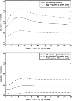
To put the subsequent discussion in the proper empirical con-text, Figure 1 presents the estimated IRFs based on the lev-els and differenced specifications with quarterly U.S. data for the period 1948:Q2–2005:Q3. U.S. data on labor productivity, hours worked in the nonfarm business sector, and population over age 16 years are obtained from DRI Basic Economics (the mnemonics are LBOUT, LBMN and P16, respectively). The difference in the IRFs is quite striking. Despite the voluminous recent literature on the effects of technology shock on hours worked, how such large quantitative and qualitative differences in the impulse responses can be generated remains poorly un-derstood. Whereas the literature attributes these discrepancies to potential biases in both VAR specifications, it is not clear that such biases are sufficiently large in practice to explain such highly divergent results, especially in the short run. In fact, we find that it is nearly impossible to justify these differences solely by the behavior of hours worked itself and, in particular, by small deviations of the largest root of hours worked from unity.
It is well known, for example, that overdifferencing, and mis-specification in general, can lead to biased results. However, what is indeed surprising is that a seemingly very minor (even undetectable) misspecification in the difference specification, may lead to a very substantial bias in the resulting IRF. Stan-dard unit root and stationarity tests on hours worked, neither of
Figure 1. Response of hours worked to a 1% positive technology shock, U.S. data 1948:Q2–2005:Q3. Top: Hours worked in levels. Bot-tom: Hours worked in first differences.
which reject their respective null hypothesis, provide little guid-ance regarding this choice of specification (Christiano, Eichen-baum, and Vigfusson2006). Pesavento and Rossi (2005) pro-vided confidence intervals on the largest autoregressive (AR) root in hours worked using inversions of four different unit root tests. All four confidence intervals include unity, and in two cases, the lower bound on the largest root exceeds 0.980; in the other two cases, it exceeds 0.925. On the face of it, this hardly appears to be a case in which overdifferencing would lead to large misspecification errors. In fact, in a reduced-form near-unit root model, the specification error that arises from overdif-ferencing is second-order. Nevertheless, Christiano, Eichen-baum, and Vigfusson (2003) reported quite a large specification error in their calibrated simulations. This provocative result has yet to be satisfactorily explained in an econometric sense.
Another way to look at the problem is to note that the dif-ferenced specification ignores possible low-frequency comove-ments between labor productivity growth and hours worked. Figure2shows that the HP trend of labor productivity growth and hours worked exhibit some similarities and suggest that la-bor productivity growth might inherit its small low-frequency trend component from hours worked. On a more intuitive level, if hours worked follow a highly persistent, but station-ary, process, it is possible that labor productivity growth
inher-its some small low-frequency component from hours without inducing any observable changes in its time series properties.
In fact, as we show later, the seemingly conflicting evi-dence from the levels and differenced specifications identified with LR restrictions can be reconciled only when these devi-ations from the exact unit root are accompanied by small low-frequency comovements between labor productivity growth and hours worked. We show that this low-frequency comovement drives a wedge between the levels and differenced specifica-tions with a profound impact on their IRFs.
This situation arises when restrictions on the matrix of LR multipliers, which includes low-frequency information, are used to identify technology shocks. Whereas the levels specifi-cation explicitly estimates and incorporates this low-frequency comovement in the computation of the impulse response func-tions, the differenced specification restricts this element to be 0. It is important to emphasize that this component could be arbitrarily small and could accompany an AR root arbitrarily close to 1, yet still produce substantial differences in the im-pulse responses from the two specifications. Thus our results also suggest that a pretesting procedure for a unit root will be ineffective in selecting a model that closely approximates the true IRF when hours worked are close to a unit root process. In this case, the pretesting procedure would favor the differ-enced specification, which rules out the aforementioned low-frequency correlation, with high probability. This in turn could result in highly misleading IRF estimates. In the next section, we provide more formal arguments for explaining and recon-ciling the conflicting empirical evidence from the levels and differenced specifications.
3. ANALYTICAL FRAMEWORK FOR UNDERSTANDING THE DEBATE
Our analytical framework and econometric specification is designed to mimic some of the salient features of the data and the implications of the theoretical macroeconomic models, par-ticularly RBC models. First, we specify labor productivity as an exact unit root process. The RBC model imposes a unit root on technology, and the data provide strong empirical support for this assumption. Hours worked exhibit a highly persistent, near-unit root behavior, although the standard RBC model im-plies that they are a stationary process. Because an exact unit root cannot be ruled out as an empirical possibility, we do not take a stand on this issue and consider both the stationary and unit root cases. However, these different specifications (sta-tionary and nonsta(sta-tionary) either allow for or restrict the low-frequency comovement between hours worked and labor pro-ductivity growth. It turns out that this has crucial implications for the IRFs.
If hours worked are stationary, then the matrix of largest roots of the labor productivity growth and hours worked can contain a nonzero upper off-diagonal element, whose magnitude depends on the closeness of the root of hours worked to 1. This typically fairly small off-diagonal element can produce substantial dif-ferences in the shapes and the impact values of the IRFs from models that incorporate (levels specification) or ignore (differ-enced specification) this component.
Figure 2. HP trends of labor productivity growth (top) and hours worked (bottom), U.S. data 1948:Q2–2005:Q3.
If hours worked have an exact unit root, the matrix of largest roots specializes to the identity matrix. In this case, there can be no low-frequency comovement between hours worked and labor productivity growth, ruling this out as an explanation for the difference between the two sets of IRFs. It is important to note, however, that this explanation is ruled out only in the case of an exact unit root. Our results suggest that this small low-frequency comovement can continue to induce large discrepan-cies between the IRFs of the differenced VARS and the levels VARs, even when the largest root is arbitrarily close to and in-distinguishable from unity.
To complete the model, we need to adopt an identification scheme that allows us to recover the structural parameters and shocks. We follow the literature and impose the LR identifying restriction that only shocks to technology can have a perma-nent effect on labor productivity. In addition, we assume that the structural shocks are orthogonal. In the following sections, we formalize this analytical framework and work out its impli-cations for the IRFs based on levels and differenced specifica-tions.
3.1 Reduced-Form Model
Consider the reduced form of a bivariate VAR processyt=
(lt,ht)′of orderp+1
(L)(I−L)yt=ut, (1) where E(ut|ut−1,ut−2, . . .)=0, E(utu′t|ut−1,ut−2, . . .)=, suptE[ut2+ξ]<∞forξ >0,and
(L)=I−
p
i=1 iLi=
ψ11(L) ψ12(L)
ψ21(L) ψ22(L)
is a finite-order lag polynomial whose roots lie strictly outside the unit circle. The matrixcan be expressed in terms of its eigenvalue decomposition as=V−1V, where=1
0 0 ρ
contains the largest roots of the system and V=10 −1γ is a matrix of corresponding eigenvectors (see, e.g., Pesavento and Rossi2006). Simple algebra yields=1
0 δ ρ
, whereδ= −γ (1−ρ)is the parameter that determines the low-frequency comovement between the variables andρ denotes the largest root of hours worked.
This parameterization, which arises directly from the eigen-value decomposition of, allows for a small (δ) impact ofhton
lt, provided thatρis not exactly equal to 1. Note that in the
ex-act unit root case,collapses to the identity matrix. The other off-diagonal element ofV, and thus of, is set to 0, because otherwise it would imply that hours isI(2)whenρ=1 andI(1)
whenρ <1.In principle, the model also can be generalized to include a nonzero (but asymptotically vanishing) feedback from the level of productivity to hours worked. Simple algebra (avail-able from the authors on request) shows that this parameteriza-tion does not materially affect our subsequent analysis. For this reason, we set the lower off-diagonal element ofto 0 with-out any loss of generality. It is important to note, however, that the zero lower off-diagonal restriction on matrix does not rule out feedback from productivity growth to hours worked in higher-order (p>1) VAR models. Thus it has no implica-tion for the direcimplica-tion of causality implied by the low-frequency correlation between hours worked and productivity growth. For example, in a VAR(2)model, the lagged productivity growth is allowed to affect hours worked through the possibly nonzero coefficientsψ21(L).
It is convenient to rewrite model (1) in the framework of Blanchard and Quah (1989) by imposing the exact unit root on productivity so that△ltis a stationary process. In this case, let
yt=(△lt,ht)′ and A(L)=(L)
Then the reduced form VAR model is given by
A(L)yt=ut (2)
or yt =A1yt−1+ · · · +Ap+1yt−p−1+ut. The nonzero
off-diagonal elementγ (1−ρ)L allows for the possibility that a small low-frequency component of hours worked affects labor productivity growth. When the low-frequency component is re-moved from either hours worked (Francis and Ramey 2009; Gali and Rabanal2004) or labor productivity growth (Fernald
2007), this coefficient is driven to 0 and the estimated IRF re-sembles the IRF computed from the differenced specification. The foregoing parameterization ofcan be used to explain this result.
3.2 Structural VAR
We denote the structural shocks (technology and nontechnol-ogy shocks) byεt=(εzt, εd
t)′, respectively, which are assumed
to be orthogonal with variancesσ12andσ22, and relate them to
Premultiplying both sides of (2) by the matrixB0and defining
B(L)=B0A(L)yields the SVAR model
B(L)yt=εt.
The matrix of LR multipliers in the SVAR forytis
B(1)=
Imposing the restriction that nontechnology shocks have no per-manent effect on labor productivity renders the matrix B(1)
lower-triangular. Forρ <1, this LR restriction translates into the restrictionb(120)= [γ ψ11(1)+ψ12(1)]/[γ ψ21(1)+ψ22(1)]. and even if the upper-right element ofis nonzero, the differ-enced VAR would ignore any information contained in the level ofht−1by implicitly setting this element to 0.
Once the structural parameter b(120) is obtained (by plugging consistent estimates of the elements of(1)from the reduced-form estimation), the remaining parameters can be recovered fromB0E(utu′t)B′0=E(εtε
where ij is the[ij]th element of. These parameters can be
used for impulse response analysis and variance decomposition.
3.3 Implications for Impulse Response Analysis
The IRFs of hours worked to a shock in technology can be computed either from the levels specification or the differenced specification. The levels approach will explicitly take into ac-count and estimate a possible nonzero upper off-diagonal ele-ment in, but it suffers from some statistical problems when hours worked are highly persistent. Christiano, Eichenbaum, and Vigfusson (2003) note that the levels specification tends to produce IRFs with large sampling variability that are nearly uninformative for distinguishing between competing economic theories. Gospodinov (2010) showed that this large sampling uncertainty arises from a weak instrument problem when the largest root of hours worked is near the nonstationary bound-ary. On the other hand, the differenced approach will produce valid and asymptotically well-behaved IRF estimates in the ex-act unit root case, but it ignores any possible low-frequency co-movement between hours and labor productivity growth when hours worked is stationary. Thus it can give rise to highly mis-leading IRFs even for very small deviations from the unit root assumption on hours.
Becauseb(120)= [γ ψ11(1)+ψ12(1)]/[γ ψ21(1)+ψ22(1)]and
b(120)=ψ12(1)/ψ22(1)can produce very different values ofb(120), the IRFs from these two approaches can be vastly different. In fact, because the value of γ does not depend onρ, these dif-ferences can remain large even for(ρ−1)arbitrarily close, but not equal, to 0. For simplicity, take the first-order model where (L)=I. In this case the two restrictions set the value ofb(0) 12 toγ and 0, respectively, implying two very different values for
b(210), which in turn directly determines the IRF. In particular, in the first-order model the impulse response of hours at timet+k
to a unit shock in technology at timetis given by
[kB−1 the debate on the distance ofρfrom 1 is misleading, provided thatρis not precisely equal to 1.
Interestingly, the differences between the IRFs do not neces-sarily disappear as ρ gets closer to 1 andδ approaches 0. As
our analytical framework suggests, they can remain substantial even for values ofρ−1 andδ= −γ (1−ρ)arbitrarily close to, but not equal to, 0. This is because, provided thatρ <1, the size of this discrepancy depends on the comovement through the parameterγ, rather than through eitherδorρ. At a more intu-itive level, the reason that the short-horizon IRFs can be highly sensitive to even small low-frequency comovements accompa-nying small deviations ofρ from 1, is that they are identified off of LR identification restrictions, which depend entirely on the zero-frequency properties of the data. As we report later, a similar sensitivity does not arise when short-run identification restrictions are applied.
3.4 An Alternative Parameterization
The fact that our framework suggests potentially large IRF discrepancies even for values ofρquite close to 1 is practically relevant, precisely because this is the case in which unit root tests have the greatest difficulty in detecting stationarity. The low power of the unit root test in this case arises because, in small samples, the resulting process for hours may behave more like a unit root process than like a stationary series. This con-cept has been formalized in the econometrics literature by the near unit root or local-to-unity model, in whichρ=1−c/T
for c≥0 is modeled as a function of the sample sizeT and shrinks toward unity asTincreases (Phillips1987; Chan1988). Naturally, this dependence on sample size should not be inter-preted as a literal description of the data, but rather as a device to approximate the behavior of highly persistent processes in small samples. What makes this modeling device particularly relevant, is that for small values of the local-to-unity parameter
c, it describes a class of alternatives toρ=1 against which unit root tests have no consistent power. Intuitively,c=T(1−ρ)
can be viewed as measuring the distance of the root from 1 rel-ative to the sample size. Small values ofccorrespond to cases in whichT is relatively small andρis relatively close to 1, so that unit root tests have low power and the difference specification is likely to be used when computing IRFs.
Thus an alternative parameterization of the model in (1) is obtained by modeling the largest root in hours as a local-to-unity process withρ=1−c/Twithc≥0. It then follows that
In finite samples, as long asc>0, the feedback from hours to productivity is nonzero, yet arbitrarily small. The reduced form foryt=(△lt,ht)′is now
In the unit root case (c=0),Tcollapses to the identity matrix, the variables are not cointegrated, and there is no feedback from hours to productivity growth. Thus the impact ofht−1on△ltis
local-to-zero and vanishing at rateT−1/2, because the level of
haffects△ltthrough the term(γc/T)ht−1, which isOp(T−1/2)
following thatT−1/2ht−1=Op(1)in the local-to-unity setup.
This captures the notion that the low-frequency comovement between hours and productivity growth must be small if the root of hours is close to unity. Writing the model in the local-to-unity form is also intuitively appealing, because the low-frequency correlation betweenht−1and△ltis bound to disappear
asymp-totically, so that hours do not affect productivity growth in the long run.
Under the local-to-unity parameterization, the matrix of LR multipliers becomes
and the restriction that nontechnology shocks have no per-manent effect on labor productivity yieldsb(120)= [γ ψ11(1)+
ψ12(1)]/[γ ψ21(1)+ψ22(1)] for c>0. Note that when c= 0, the model again specializes to the differenced VAR spec-ification in (3), for which the LR restriction implies b(120) =
ψ12(1)/ψ22(1). As a result, the analysis of the shapes of the IRFs under the different specifications in Section3.3remains unchanged. This confirms our finding that substantial differ-ences in IRFs can arise even within this class of models for which unit root tests are not sufficiently powerful to detect that hours worked are stationary. Thus the stylized fact that hours worked are indistinguishable from a unit root process does not guarantee that the true IRF will be close to the IRF from the differenced specification.
4. MONTE CARLO EXPERIMENT
To demonstrate the differences in the IRF estimators with a nondiagonal,we conducted a Monte Carlo simulation exper-iment. We generated 10,000 samples foryt=(lt,ht)′ from the
, and the parameter values are calibrated to mimic the empirical shape of the IRF of hours worked to a technology shock. Note that whereas the numbers for the short-run dynam-ics are chosen to match the values estimated from a VAR in lev-els, in our simulations we consider bothρ <1 andρ=1 and thus allow both specifications (levels and first differences) to be the true data-generating process. The lag order of the VAR is assumed known. In addition to the IRF estimates from the levels and differenced specifications, we consider the IRF esti-mates from a levels specification with HP detrended productiv-ity growth, as was done by Fernald (2007). We set the smooth-ing parameter for the HP filter to 1600.
Figures3–5show simulation results for the IRFs under three different parameter configurations forρandγ, all of which lie in a range of values that is potentially consistent with the actual data. The three panels of each figure correspond to the different model specifications: a VAR in productivity growth and hours, a VAR in productivity growth and differenced hours, and a VAR in HP detrended productivity growth and hours. For each model
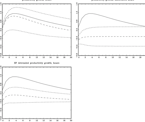
Figure 3. Response of hours to a positive technology shock (LR identification) with data simulated from the model[I−−00..205 −00.55.08L] × [I−10 ρδL]lt
ht
=u1,t
u2,t
,whereρ=0.95, δ=0.04 (γ= −0.8),(u1,t,u2,t)′∼iid N(0,),=
0.78 0
0 0.55
andT=250.The solid line represents true IRF; the long-dashed line,median Monte Carlo IRF estimate; the short-dashed line, 95% Monte Carlo confidence bands.
we show the true IRF (solid line), the median Monte Carlo IRF estimate (long-dashed line), and the 95% Monte Carlo confi-dence bands (short-dashed line).
In Figure3 we consider a stationary but persistent process for hours (ρ =0.95), while allowing a small low-frequency component of hours worked to enter labor productivity growth (δ =0.04). As shown in the figure, the VAR in levels (left graph) estimates an IRF that is close on average to the true IRF, except for a small bias (see Gospodinov2010for an explana-tion). On the other hand, the VAR with hours in first differences (middle graph) incorrectly estimates a negative initial impact of the technology shock even though the true impact is positive. This demonstrates the ability of even a small low-frequency co-movement to drive a qualitatively important wedge between the IRFs based on the levels and differenced models.
The lower panel of Figure3also provides interesting infor-mation. When the HP filter is used to remove the low-frequency component from labor productivity growth (Fernald2007), the
estimated IRF resembles the IRF computed from the differ-enced specification. The graphs clearly demonstrate that re-moval of the low-frequency component either by differenc-ing or by HP filterdifferenc-ing eliminates the possibility of any low-frequency comovements between the transformed series, which has a profound influence on the IRFs. We also considered the specification when hours worked are HP-filtered, as was done by Francis and Ramey (2009). The behavior of the IRF esti-mates in this model is similar to the case of HP-filtered produc-tivity growth.
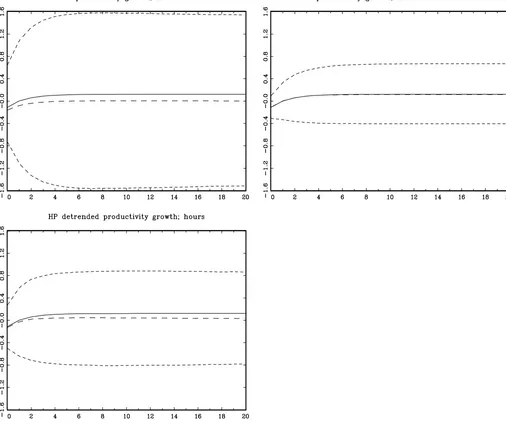
Figure4presents the results for the exact unit root case. In this case the matrix of largest roots becomes diagonal, elimi-nating the low-frequency comovement between hours and pro-ductivity growth (δ =0). Despite some small biases, all me-dian IRF estimates now correctly sign the impact of the tech-nology shock and come close to tracing out the true IRFs. Not surprisingly, the differenced specification is particularly accu-rate and produces an unbiased estimator with tight confidence
Figure 4. Response of hours to a positive technology shock (LR identification) with data simulated from the model[I−−00..205 −00.55.08L] × [I−10 ρδL]lt
ht
=u1,t
u2,t
,whereρ=1, δ=0 (γ=0),(u1,t,u2,t)′∼iid N(0,),=
0.78 0
0 0.55
andT=250.The solid line represents the true IRF; the long-dashed line, median Monte Carlo IRF estimate; the short-dashed line, 95% Monte Carlo confidence bands.
intervals. The estimator from the levels specification exhibits both a modest bias that arises from the biased estimation of the largest root of hours and a very large sample uncertainty (Gospodinov2010). The estimator using HP-filtered labor pro-ductivity growth performs similarly to the differenced estima-tor, although it is slightly biased and more dispersed.
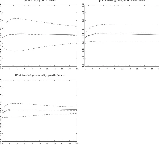
In Figure 5 we maintain the assumption of a zero off-diagonal element (δ=0) and return to a persistent but station-ary specification for hours worked (ρ=0.95). The median IRFs from all models again are quite similar both to one another and to the true IRF. In this sense, besides having smaller bias and variance, the basic message from Figures 4 and5 is similar, despite the fact that hours are nonstationary in Figure4but sta-tionary in Figure5.
In summarizing the results from these three figures, we note that large qualitative differences in median IRFs for the differ-enced and levels VARs are seen only in Figure3, in which there is a small low-frequency relationship between hours and labor
productivity (δ=0). Neither Figure4nor Figure5shows qual-itative differences in the median IRFs from the levels and dif-ferenced specifications. Yet in Figure4, hours have a unit root, whereas in Figure5they are stationary. Although small sample bias is present and affects the precision of the estimation, our simulations show that the small sample bias and persistence of the nontechnology shocks alone are not sufficient to generate the substantial differences in impulse responses that we find in practice. What Figures4and5share in common is the absence of the low-frequency comovement of Figure3. Although the size of the unit root in hours worked has important implica-tions for the sampling distribuimplica-tions of the IRFs, these results suggest that the low-frequency comovement plays the critical role in driving the qualitative differences between the level and differenced specifications.
We also want to stress that the confidence intervals reported in Figures 3–5 are Monte Carlo confidence intervals, which
Figure 5. Response of hours to a positive technology shock (LR identification) with data simulated from the model[I−−00..205 −00.55.08L] × [I−10 ρδL]lt
ht
=u1,t
u2,t
,whereρ=0.95, δ=0 (γ=0),(u1,t,u2,t)′∼iid N(0,),=
0.78 0
0 0.55
andT=250.The solid line represents true IRF; the long-dashed line, median Monte Carlo IRF estimate; the short-dashed line, 95% Monte Carlo confidence bands.
are infeasible because they use knowledge of the true data-generating process. The bias in the levels VAR and the mis-specification in the first-difference regressions result in poor coverage of confidence intervals constructed with standard pro-cedures at medium and long horizons (Pesavento and Rossi
2006). This is not reflected in our infeasible confidence inter-vals. Nonetheless, Figures3 and 4 clearly show how a wide range of different estimates for the IRF are possible, and that the sampling uncertainty in the levels VAR is indeed larger. At the same time, except for the cases in which eitherρ is exactly 1 orδ is exactly 0, the true impulse response is never contained in the Monte Carlo confidence bands for the VAR in first differ-ences.
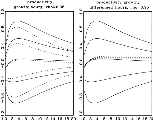
To better assess the sensitivity of the levels and differenced specifications to different values ofδ, Figure 6 plots the true
and estimated responses for ρ=0.95 and various degrees of low-frequency comovement. Each line represents values for
γ = {−0.5,−0.2,0,0.2,0.5}, which correspond to different off-diagonal elementsδdepending on the value ofρ[recall that
δ= −γ (1−ρ)]. Once again, it is clear that whereas the level specification explicitly estimates and incorporates the different values for δ in the computation of the IRFs, the differenced specification implicitly imposes this element to be 0. This leads to substantial deviations from the true IRFs.
Finally, the differences in the IRFs for the various model specifications are expected to arise only in the case of LR iden-tification restrictions that are directly affected by the inclusion or the omission of the low-frequency component. To verify this conjecture, we estimate the IRFs based on a short-run iden-tification (Choleski decomposition) scheme, with productivity
Figure 6. Response of hours to a positive technology shock (LR identification) with data simulated from the model [I −
−0.05
and T =250. The solid line represents true IRF; the short-dashed line, median Monte Carlo IRF estimate.
growth ordered first and hours ordered second. We emphasize that our short-run identifying scheme is used only to illustrate the relative insensitivity of the IRFs to the low-frequency co-movement when they are identified by short-run restrictions. We do not advocate its use in practice, because it has no clear theoretical justification. (See Christiano, Eichenbaum, and Vig-fusson2006for a more sophisticated, model-based, short-run identification scheme.)
Figure7presents the results from the three models forρ= 0.95 andδ=0.04. Unlike the LR identification scheme (Fig-ure3), the IRF estimates for all specifications are very close to the true IRF and fall inside the 95% Monte Carlo confidence bands. This suggests that the short-run identification scheme is robust to the presence or absence of low-frequency comove-ments, which is not the case with identifying restrictions based on LR information.
The simulation results so far were obtained under the main-tained hypothesis of an underlying low-frequency comovement in the data forδ=0, which is implicitly assumed to be struc-tural in nature. An online Appendix (available on the authors’ Web pages) presents additional simulation results from two ob-servationally equivalent structural break models that give rise to the common high-low-high pattern observed by Fernald (2007). These simulations are intended to provide some insight into the underlying reasons for the differences between our results and the results of Fernald (2007). These results clearly indicate that imposing the assumption that the timing of the breaks is co-incidental (Fernald2007) or exogenously driven (Francis and Ramey2009) is crucial for producing evidence supporting the break removal or HP filtering before the IRF analysis as ad-vocated by Fernald (2007) and Francis and Ramey (2009). In contrast, the results from a cobreak model, where the similar magnitude and timing of the breaks is driven by a common un-derlying component, are qualitatively similar to those presented
herein, in which removing the low-frequency component leads to substantial deviations of the IRF estimates from their true values.
5. DISCUSSION
The analytical and numerical results presented herein clearly suggest that some seemingly innocuous transformations of the data can lead to vastly (qualitatively and quantitatively) differ-ent policy recommendations. The main objective of this arti-cle is to illustrate and identify the source of these differences. At the same time, several interesting observations and remarks emerge from our analysis that highlight some potential pit-falls in empirical work with structural dynamic models that use highly persistent variables in conjunction with LR identifying restrictions. Following Blanchard and Quah (1989), LR iden-tifying restrictions have been popular tools in applied macro-economics (see, e.g., Rogers1999; Lastrapes1992; Clarida and Gali1994), whereas ever since the work of Nelson and Plosser (1982), the low-frequency properties of macroeconomic data series have been widely debated. Thus these more general in-sights are likely to be useful in other contexts as well.
First, it is common practice in macroeconomics to remove low-frequency components by applying the HP filter when fo-cusing on business cycle frequencies. For example, Fernald (2007) argued that the low-frequency component is not im-portant for business cycle analysis. The effect of technology shocks on hours worked is typically evaluated at business cy-cle frequencies, and it is reasonable to assume that the removal of low-frequency components will not affect the conclusions. We agree with this position, provided that the structural shocks are identified using short- or medium-run restrictions. We argue that the low-frequency component contains important LR in-formation that, although not directly relevant at business cycle frequencies, affects the LR restrictions in a fundamental way. Thus omitting or explicitly removing the low-frequency corre-lation can result in misspecification of the LR restriction and hence the business cycle component that is of primary inter-est to the analysis. In contrast, the low-frequency component does not seem to matter for the short-run restrictions, and the transformations applied to the data do not affect the impulse responses that they identify, as we have illustrated in our simu-lations.
Although the analogy is not exact, the removal of low-frequency components has some similarities to ignoring the LR information contained in the error-correction term in cointe-grated models. The cointegration information does not directly affect the business cycle analysis, but is essential to the LR equilibrium. If we use short-run restrictions, then the cointegra-tion informacointegra-tion can be omitted without serious consequences. If the data are subjected to differencing (filtering) before the analysis, then the LR information contained in the cointegrat-ing relationship is lost and the LR restriction is misspecified, which in turn gives rise to misleading results.
Second, it is well known that a highly persistent linear process often exhibits dynamics that are observationally equiv-alent to the dynamics generated by a long memory, structural break, or regime-switching process. Consequently, it is diffi-cult to statistically distinguish between these processes in finite
Figure 7. Response of hours to a positive technology shock [short-run (Choleski) identification] with data simulated from the model
[I−−00..205 −00.55.08L][I−10 δρL]lt
ht
=u1,t
u2,t
, whereρ=0.95, δ=0.04 (γ = −0.8),(u1,t,u2,t)′∼iid N(0,),=
0.78 0.1
0.1 0.55
and T=250.The solid line represents true IRF; the long-dashed line, median Monte Carlo IRF estimate; the short-dashed line, 95% Monte Carlo confidence bands.
samples and to commit to a particular specification. In our con-text, determining whether or not the low-frequency component (e.g., the U-shape in hours worked) and comovement are spuri-ous is difficult. Fernald (2007) convincingly illustrated the cost of falsely keeping the low-frequency component if this comove-ment is spurious. Our results indicate that there is an equally large cost of falsely removing it when the comovement is a true feature of the correctly identified model. Ultimately, the researcher must take a stand on whether the LR restriction ap-plies to the original or filtered data. Our analysis in the previous sections provides important information on the sensitivity (ro-bustness) of the different statistical transformations of the data to misspecification of the LR restriction.
Finally, pretesting procedures that are used to determine which specification is more appropriate perform poorly, espe-cially when the data are highly persistent. Our analysis suggests
that large differences in the IRFs arise even when the largest root is arbitrarily close to 1, in which case the pretesting pro-cedure selects the differenced specification with probability ap-proaching 1. Put another way, we find that when identified by LR restrictions, the IRFs from the differenced specification are not robust to small deviations of the largest root from unity, even when those deviations are too small to be empirically de-tected.
6. CONCLUSION
This article analyzes the source of the conflicting evidence from structural VARs identified by LR restrictions on the effect of technology shocks on hours worked reported in several re-cent empirical studies. We show analytically that the extreme sensitivity of the results to different model specifications can
be explained by a discontinuity in the solution for the struc-tural coefficients implied by the LR restrictions, which arises only in the presence of a low-frequency correlation between hours worked and productivity growth. The critical mechanism underlying the difference between the levels and differenced specifications is that the differenced specification restricts this correlation to 0 when solving for structural model, whereas the levels specification allows it to enter in an unrestricted manner. Consequently, it may not be surprising that alternative filter-ing approaches reported in the literature, such as HP filterfilter-ing and trend-break removal, which eliminate this low-frequency correlation, provide evidence supporting the differenced VAR. We also demonstrate that low-frequency correlations capable of causing strong discrepancies between the two specifications are compatible with AR roots in hours worked that are indis-tinguishable from 1. This sharp discontinuity implies that one cannot rely on univariate unit root tests to resolve this debate, because they are not designed to discriminate between exact and near-unit root models.
Fernald (2007) also highlighted the role of an observed low-frequency correlation in the data, modeled as a common U-shaped pattern driven by structural breaks, and provided some convincing empirical exercises to illustrate its impor-tance. Although that insightful analysis clearly demonstrated the empirical link between the low-frequency correlation and the conflicting results, a full theoretical understanding of why this low-frequency correlation plays such an important role re-mains elusive. We fill this gap by showing, in a more general an-alytic framework, that the key role played by this low-frequency correlation is to create a discontinuity between the structural so-lutions of the differenced and levels specifications.
We argue that the importance of the low-frequency correla-tion cannot by itself resolve the debate, because, depending on the way in which it is modeled, it may lead to biases in either the levels or differenced specification. However, in conjunction with the work of Fernald (2007) and Francis and Ramey (2009), our results help clarify the terms of the debate. We demon-strate that if there is a true low-frequency correlation in the population model that is correctly identified by the LR iden-tification restriction, then any procedure that removes this low-frequency correlation, whether by differencing, HP filtering, or trend-break removal, would result in a substantial bias. In fact, we find that we cannot reproduce the discrepancy in the results with any reasonable probability in a correctly identified model without introducing such a true population correlation.
The reason why this finding might seem to be at odds with the results of Fernald (2007) and Francis and Ramey (2009), who argued that the levels specification is biased, is that neither of those authors perceived the observed correlation as an inher-ent feature of the correctly idinher-entified model. Fernald (2007) ar-gued that the observed low-frequency correlation is purely co-incidental and that a similar pair of breaks in both series oc-curs due to historical happenstance. Francis and Ramey (2009) treated the observed correlation as a population characteristic explained by common low-frequency trends in demographic and public employment, but argued that the LR restriction does not hold until these low-frequency trends are purged from the data. In our view, the debate thus hinges on the interpretation given to this low-frequency correlation. If one has reason to be-lieve that there is a genuine low-frequency comovement in a
correctly identified model, then this would support the findings of Christiano, Eichenbaum, and Vigfusson (2003). On the other hand, if one is convinced either that the observed correlation is coincidental (Fernald2007) or that it is due to factors that vi-olate the identification restriction (Francis and Ramey2009), then the results may be interpreted as supporting the earlier findings of Gali (1999). More generally, our results help explain the empirically observed sensitivity of LR identifying schemes to uncertainty regarding low-frequency dynamics, even when identifying characteristics at business cycle frequencies.
ACKNOWLEDGMENTS
The authors thank the Editor (Jonathan Wright), an Asso-ciate Editor, two anonymous referees, Michelle Alexopolous, Efrem Castelnuovo, Yongsung Chang, Francesco Furlanetto, Leo Michelis, Barbara Rossi, Shinichi Sakata, seminar partic-ipants at University of Padova, University of Cyprus, sity of British Columbia, Carleton University, Queens Univer-sity and Louisiana State UniverUniver-sity and conference participants at the 2008 Far Eastern Meetings of the Econometric Society, the 2008 Meeting of the Canadian Econometric Study Group, ICEEE 2009, CIREQ Time Series Conference and the 2009 Joint Statistical Meetings for helpful comments and sugges-tions. Part of this research was done while Elena Pesavento was a Marco Fanno visitor at the Dipartimento di Scienze Economiche at Universita’ di Padova. Nikolay Gospodinov gratefully acknowledges financial support from FQRSC and SSHRC.
[Received February 2010. Revised October 2010.]
REFERENCES
Alexopoulos, M. (2011), “Read All About It! What Happens Following a Tech-nology Shock?”American Economic Review, 101, 1144–1179. [455] Basu, S., Fernald, J. G., and Kimball, M. S. (2006), “Are Technology
Improve-ments Contractionary?”American Economic Review, 95, 1418–1448. [455] Blanchard, O., and Quah, D. (1989), “The Dynamic Effects of Aggregate De-mand and Supply Disturbances,”American Economic Review, 79, 655–673. [459,464]
Chan, H. C. (1988), “The Parameter Inference for Nearly Nonstationary Time Series,”Journal of the American Statistical Association, 83, 857–862. [460] Chang, Y., Hornstein, A., and Sarte, P.-D. (2009), “On the Employment Effects of Productivity Shocks: The Role of Inventories, Demand Elasticity, and Sticky Prices,”Journal of Monetary Economics, 56, 328–343. [455] Chari, V., Kehoe, P., and McGrattan, E. (2008), “Are Structural VARs With
Long-Run Restrictions Useful in Developing Business Cycle Theory?”
Journal of Monetary Economics, 55, 1337–1352. [456]
Christiano, L., Eichenbaum, M., and Vigfusson, R. (2003), “What Happens After a Technology Shock?” International Finance Discussion Paper 768, Board of Governors of the Federal Reserve System. [455-457,459,466]
(2006), “Assessing Structural VARs,” inNBER Macroeconomics An-nual, eds. D. Acemoglu, K. Rogoff, and M. Woodford, Cambridge: MIT Press. [455-457,464]
Clarida, R., and Gali, J. (1994), “Sources of Real Exchange Rates Fluctuations: How Important Are Nominal Shocks?”Carnegie-Rochester Conference Se-ries in Public Policy, 41, 1–56. [464]
Erceg, C., Guerrieri, L., and Gust, C. (2005), “Can Long-Run Restrictions Iden-tify Technology Shocks?”Journal of the European Economic Association, 3, 1237–1278. [456]
Fernald, J. (2007), “Trend Breaks, Long-Run Restrictions, and Contractionary Technology Improvements,”Journal of Monetary Economics, 54, 2467– 2485. [455,456,459-461,464-466]
Francis, N., and Ramey, V. (2005), “Is the Technology-Driven Real Business Cycle Hypothesis Dead? Shocks and Aggregate Fluctuations Revisited,”
Journal of Monetary Economics, 52, 1379–1399. [455]
(2009), “Measures of Hours Per Capita With Implications for the Technology-Hours Debate,”Journal of Money, Credit, and Banking, 41, 1071–1097. [456,459,461,464,466]
Francis, N., Owyang, M., and Roush, J. (2005), “A Flexible Finite-Horizon Identification of Technology Shocks,” Working Paper 2005-024E, Federal Reserve Bank of St. Louis. [455]
Gali, J. (1999), “Technology, Employment, and the Business Cycle: Do Tech-nology Shocks Explain Aggregate Fluctuations?”American Economic Re-view, 89, 249–271. [455,456,466]
Gali, J., and Rabanal, P. (2004), “Technology Shocks and Aggregate Fluctua-tions: How Well Does the RBC Model Fit Postwar U.S. Data?” inNBER Macroeconomics Annual, eds. B. Bernanke and K. Rogoff, Cambridge: MIT Press. [455,459]
Gospodinov, N. (2010), “Inference in Nearly Nonstationary SVAR Models With Long-Run Identifying Restrictions,”Journal of Business & Economic Statistics, 28, 1–12. [459,461,462]
Lastrapes, W. D. (1992), “Sources of Fluctuations in Real and Nominal Ex-change Rates,”Review of Economic and Statistics, 74, 530–539. [464]
Nelson, C., and Plosser, C. (1982), “Trends and Random Walks in Macroeco-nomic Time-Series: Some Evidence and Implications,”Journal of Monetary Economics, 10, 139–162. [464]
Pesavento, E., and Rossi, B. (2005), “Do Technology Shocks Drive Hours Up or Down? A Little Evidence From an Agnostic Procedure,”Macroeconomic Dynamics, 9, 478–488. [457]
(2006), “Small Sample Confidence Intervals for Multivariate Impulse Response Functions at Long Horizons,”Journal of Applied Econometrics, 21, 1135–1155. [458,463]
Phillips, P. C. B. (1987), “Towards a Unified Asymptotic Theory for Autore-gression,”Biometrika, 74, 535–547. [460]
Ravenna, F. (2007), “Vector Autoregressions and Reduced Form Representa-tions of DSGE Models,”Journal of Monetary Economics, 54, 2048–2064. [456]
Rogers, J. H. (1999), “Monetary Shocks and Real Exchange Rates,”Journal of International Economics, 49, 269–288. [464]
Shea, J. (1999), “What Do Technology Shocks Do?” inNBER Macroeconomics Annual, eds. B. Bernanke and J. Rotemberg, Cambridge: MIT Press. [455] Uhlig, H. (2004), “Do Technology Shocks Lead to a Fall in Total Hours
Worked?” Journal of the European Economic Association, 2, 361–371. [455]

![Figure 7. Response of hours to a positive technology shock [short-run (Choleski) identification] with data simulated from the model� −�� 1�� l�� u�� 0�](https://thumb-ap.123doks.com/thumbv2/123dok/1151342.765840/12.594.47.564.48.483/figure-response-hours-positive-technology-choleski-identication-simulated.webp)
